Introduction

The NetFACS package is a tool that allows users to analyse and plot their facial signal data, generated using the Facial Action Coding System (FACS), in a statistical meaningful way using network analysis. FACS data, based on the co-occurrence of different elements representing facial muscle movements (called ‘Action Units’ or AUs), have some rather awkward properties: single AUs are binary (present/absent), they are part of larger expressions and combined with each other, their use can be non-normally distributed, individuals can provide multiple datapoints, data are often autocorrelated etc (see Mielke et al., 2021 for more information). NetFACS allows users to overcome some of these problems and present their results in a form that is easy to communicate to other researchers.

This is a tutorial and overview over which functions are currently available in the NetFACS package and which questions we can potentially already answer. NetFACS at this point is still work in progress. We will demonstrate the whole process of creating a NetFACS object, and explain the existing analytical and plotting tools. Currently, all functions are concerned with co-occurrence, so which elements happen simultaneously. Time-series analyses should follow soon. While we will use mainly Facial Action Coding System examples throughout (meaning ‘elements’ in the functions are Action Units, or AU), the functions can be applied to any co-occurrence data, so other questions regarding communication are also possible. This allows researchers to directly compare the complexity of different communication systems, e.g. gestures and facial expressions in nonhuman primates.

In this tutorial, we will mainly talk about FACS and emotions, simply because this has been historically the area where FACS has been employed the most. However, the main goal is to open up the use of FACS to other topics. So, whenever the ‘context’ here is ‘emotion’, any other context can be chosen: different experimental interventions, behavioural contexts, or different groups of participants.

NetFACS basics

As the name indicates, NetFACS is based on the use of networks for FACS data. Not all analyses require an understanding of networks: at its most basic, NetFACS can simply represent the probabilities that Action Units occur in a context or not, or contrast AU use between two conditions. Networks become interesting once we talk about the connections between Action Units, or the connections between AUs and contexts that goes past the pure occurrence. All analyses are based on different concepts of probability, which are explained below. Probabilities are used to quantify the strength of connection between AUs, and between AUs and contexts. The third pillar of the package, next to networks and probabilities, are two different resampling methods: permutations and bootstrapping. These are used to determine what occurrence of AUs would be expected under random circumstances or if the data were taken from a different population. We will explain their use further down, but it’s important to understand the distinction. In permutations, existing data are shuffled to create the ‘random’ probability that two AUs co-occur, for example. In bootstraps, subsets of data from a different context are selected over and over again for the same purpose.

NetFACS is based mainly on different probabilities: unconditional probability is the simply the proportion of occurrence; ). The unconditional probability of a combination AB is not directional, i.e. it is the same for AB as it is for BA: ( == ). We use the unconditional probability mainly to express how often an AU or a combination of AUs occurs at all, either in the whole data set or in a specific context. Conditional probability, on the other hand, is the probability of an event A given an event B; ). Thus, it tells us not how often A occurs at all, but how often A occurs in the subset of cases where we know that B is present. Therefore, the conditional probabilities can differ depending on which direction we are looking at ( != ). For example, in the English language, the letter ‘h’ is often accompanied by the letter ‘s’, but the reverse is not true: most cases of ‘s’ do not involve ‘h’. We can explore the conditional probability between two elements, or between an element/combination and a context. Probabilities are used as they are intuitive for most people, in contrast to many more opaque association indices that are often used in social network analysis. It also means that we can tie in other analytical tools that are very directly based on probabilities, such as Bayesian models and Markov Chains.

Install the package

Let’s start by installing the package and loading the library.

# install NetFACS from CRAN
install.packages("NetFACS")

# read library
library(NetFACS)

Alternatively, you can install the latest development version of NetFACS from GitHub with:

# install NetFACS from GitHub
devtools::install_github("NetFACS/NetFACS")

Data sets

Currently, there are two practice data sets in the package: one is the Extended Cohn-Kanade Database for posed FACS data (all basic AUs, 7 emotions) (Lucey et al. 2010), where co-occurrence is defined as Action Units happening in the same facial expression, and one is the Communist Manifesto in French, German, and English, where co-occurrence is defined as letters happening in the same word. These can be accessed the following way:

data("letternet") # this is the Manifesto #
data("emotions_set") # this is the CK Database #

Important for the NetFACS package at the moment is that the basic data used to calculate probabilities are stored in a data frame with each event as a row (this can be a communication sequence, a facial expression, a frame in a video, or a word, for example), and each element as a column (for example, Action Units in FACS data or letters for words). Elements get a 0 if they are absent in this event, and a 1 if they are present. So, for example, the word ‘word’ would have a 1 in the columns for d,o,r, and w, and 0 in all other letter columns. It’s usually good to have a second data frame of the same length that contains additional information about the condition, duration, etc. This will look like this for the words:

Letter data for words in the Communist Manifesto

Additional information for Communist Manifesto

Prepare the data

Users who code FACS data will often have them stored in a different format, where they have the Action Unit together with its start and end time or duration in a specific video. The package has a function that can deal with these data and transform them into the right format, as long as they contain information about the video from which they were taken.

So, for photos, data will sometimes look like this:

odd.photo <- data.frame(
  photo = c("photo1", "photo2", "photo3", "photo4", "photo5", "photo6"),
  AUs = c(
    "AU1/AU5/AU9",
    "AU1/AU2",
    "AU1/AU2/AU10",
    "AU1/AU2",
    "AU5/AU17/AU18",
    "AU6/AU12"
  )
)
kable(odd.photo, row.names = FALSE, caption = "Photo Data")

Photo Data

Videos, on the other hand, will sometimes look this:

odd.video <- data.frame(
  video = c(rep("video 1", 3),
            rep("video 2", 2),
            rep("video 3", 3)),
  AUs = c("AU1", "AU5", "AU9",
          "AU1", "AU2",
          "AU1", "AU2", "AU10"),
  start.times = c(0.1, 0.2, 0.3,
                  0.1, 0.3,
                  0.1, 0.4, 0.4),
  durations = rep(0.3, times = 8)
)
kable(odd.video, row.names = FALSE, caption = "Video Data")

Video Data

The prepare.netfacs() function can take either of these inputs and turn them into the right format. This will look something like this:

au.prepared <- prepare.netfacs(
  elements = odd.video$AUs,
  type = "video",
  video.id = odd.video$video,
  start.time = odd.video$start.times,
  duration = odd.video$durations,
  frame.duration = 0.05
)
kable(head(au.prepared$element.matrix),
      row.names = FALSE,
      caption = "Element Matrix of prepare.netfacs")

Element Matrix of prepare.netfacs

kable(head(au.prepared$video.info),
      row.names = FALSE,
      caption = "Video Info of prepare.netfacs")

Video Info of prepare.netfacs

The ‘netfacs’ function

The basis for the whole package so far is the ‘netfacs’ function. The function creates a list for all possible combination of elements that has the information on their observed probability of occurrence in the chosen data set. It also tests whether this observed probability is significantly different from an expected or null distribution, and gives information about the shape of that null distribution. The user defines whether this null distribution is the expected random distribution of elements (e.g., do AU1 and AU2 occur together more than expected by chance) based on permutations of the raw data that control for the overall probability of single elements occurring and the number of elements per event, or whether we are comparing two conditions (e.g., do AU1 and AU2 occur together more in sad than in angry faces) with one condition providing the null condition. In the latter case, bootstraps of the null condition are used to establish the null distribution. Bootstraps can be done by randomly selecting events, or by randomly selecting on a higher-level variable, e.g. subject, by including that variable in the ‘random.level’ parameter of the function call. For direct comparisons, one can include ‘control variables’ into the bootstrap: for example, if individual sex is included, then the bootstrap will select the null condition on the same ratio as the test condition, so if 1/3 of participants in the test condition are males, then 1/3 of cases in each random selection will also be male. This prevents biases due to sampling differences between test and null condition.

It is important to note that combination of elements here does not mean that ONLY those elements were active, but that they were among the active elements. So, the combination of AU1 + 2 is counted when the overall facial expression shows AU1+2, but also AU1+2+5, AU1+2+5+10, etc. Conditional probabilities will be based on the number of times either of the two elements were present.

NetFACS parameters

These are the function parameters and what they do:

• data: this is the data matrix that contains each event as a row and each element as a column, with 0 and 1 denoting whether an element was active at all
• condition: this denotes the condition (e.g., the emotion, language, gender …) that we want to find out about. The input should be a vector of the same length as data with the condition each event belongs to, to allow the algorithm to assign each event. If no condition is set, then all data points are compared against random distribution. If a condition is set, the user has to define a test condition: one of the levels of the condition vector that we are interested in.
• test.condition: marks the condition that we want to find out about.
• null.condition: marks the comparison level. If NULL, then the test condition is compared with all other data points (e.g. anger against all other emotions). If it is set to a value (e.g., ‘happy’), then only the test and null condition are compared with each other (e.g., happy and angry faces).
• duration: when analysing videos with FACS, each event could differ in duration; for example, some events contain 5 frames, while another contains 10 frames. If this information is available, FACS will weight the results accordingly. Here, you should enter a vector of the same length as the data set that defines the duration of each event. It doesn’t matter if you put seconds or frames as duration, the function will determine the smallest value and compare all other values to this.
• ran.trials: determines how many permutations or bootstraps are performed. The larger, the better and more accurate, but things take longer. 1000 iterations is usually good.
• control: Here, you would enter a list of control variables. So, for example, to control for gender and place of origin, you would enter ‘list(gender, place.of.origin)’; if these were available. This way, in the bootstraps, he algorithm will approximate the distribution of these control parameters in the test and null condition. So, if there are 10 males and 20 females in the angry faces, the null condition will select a ratio of 1 to 2 as well, to prevent difference to be driven by differences in the data set. Note that you need enough data to include control variables: if there are no female faces in one of the conditions, the algorithm will fail at adjusting the distribution.
• random.level: Should be a vector of the same length as the data matrix that assigns each event a higher-level identifier, such as individual or video. For the bootstraps, this works similar to a random effect in that it controls for the fact that some data points belong to the same hierachical level. So, if an individual provides several data points, or data points come from the same video, noting this in the random.level parameter means that random selection occurs on the level of the video or individual rather than each event separately. Thus, the probability space of the null distribution is not biased by one individual or video.
• combination.size: If null, the algorithm will pop out all possible combinations. If we don’t care for the higher-order combinations (e.g. combinations of 5 elements), we can speed the analysis up by limiting this to 2 or 3.
• tail: Should p-values be upper.tail (the observed value is larger than the expected values) or left.tail (the observed value is smaller than the expected values)?
• use_parallel: Should processing be done in parallel?
• n_cores: How many cores should be used for parallel processing?

Here, I will give an example where we compare the facial expression of anger against all other facial expression. We assume that every individual provided one case and there is no information about gender etc, so we do not use any controls:

Comparison of conditions

# here, we test whether any Action Units and combinations appear more frequently than expected under one condition than under another.
# load data
au.data <- emotions_set[[1]]
# this is the basic data frame, with each video represented by a row, and each Action Unit represented by a column

au.info <- emotions_set[[2]]
# this is the additional information about the emotions etc

# We remove AU 25 here, because it is not informative, and all AUs that have 2 or fewer occurrences, because not meaningful interpretation is available for them
au.data <- au.data[, setdiff(colnames(au.data), "25")]
au.data <- au.data[, colSums(au.data) > 2]

# create netfacs object for angry faces
angry.face <- netfacs(
  data = au.data, # this is the data matrix
  condition = au.info$emotion, # info about condition of each case
  test.condition = "anger", # condition we are interested in
  null.condition = NULL, # null condition (test against all other emotions)
  duration = NULL, # we could add duration information for videos
  ran.trials = 1000, # number of randomizations. The larger the better
  control = NULL, # control variables, e.g. gender, ethnicity etc.
  random.level = NULL, # Works like a random effect.
  combination.size = 4, # limit the analysis to make things faster,
  tail = "upper.tail", # should the p-value reflect two-tailed or right/left tailed testing?
  use_parallel = TRUE, # use parallel processing
  n_cores = NULL # number of cores for parallel processing
)

Top rows of the netfacs function results

Now we have the angry.face object that contains all the information we need to make networks and claims about which Action Units make up a facial expression.

As we can see in the last table already, there is a lot of information in this object:

• combination: the name of the combination
• combination.size: how many elements make up the combination
• count: how often it occurs in the test condition
• observed.prob: Probability that the combination occurs in a frame of that condition
• expected.prob: Expected probability of the combination if the data set was drawn from the null condition; mean of all randomisations.
• effect.size: Difference between the observed probability and the mean expected probability.
• pvalue: how many random probabilities were more extreme than the observed probability (larger for right.tail, smaller for left.tail)
• specificity: probability that the condition is ‘anger’ when the combination is observed. e.g, 0.8 means that 80% of all occurrences of the Action Unit are in ‘anger’
• probability.increase: how many times more likely is the combination in this condition than the null condition?

As this table is very large in many instances, we can extract results more easily while already cleaning the table a bit using the ‘extract.netfacs’ function:

# extract angry face information for the first level (single elements)
anger.aus <- netfacs_extract(
  netfacs.data = angry.face,
  combination.size = 1, # only looking at combinations with 1 element (here, Action Units)
  min.count = 1, # minimum number of times that the combination should occur
  min.prob = 0, # minimum observed probability of the combination
  min.specificity = 0, # minimum specificity of the combination
  significance = 0.01
) # significance level we are interested in

Result of netfacs_extract for single elements

The results show that in angry faces, the Action Units 4, 7, 14, 17, 18, 23, and 24 are significantly more common than would be expected given the information we have from the other emotions. AU23, for example, occurs 36 times, which is 80% of all ‘angry’ faces. Expected would be 2.5%, so we have an increase in probability of 32 times. When we see AU 23, we can be 84% sure that this is an angry face (specificity).

We can also plot this. In element.plot, the y-axis is based on the log-transformed change in probability between the observed and all randomised distributions, and the x-axis contains each element. Almost all plots that are included in the package at this point are ggplot based, so the user can subsequently change most parameters to their own liking.

# create plot showing the importance of each AU for the angry faces

element.plot(netfacs.data = angry.face)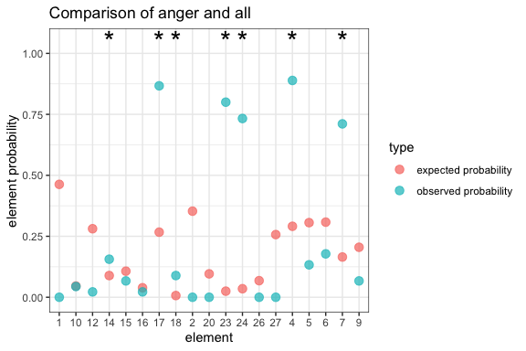

In the distribution.plot function, we see the distribution of the null probabilities and where the observed values fall in comparison. It does this independently for each element. Here, we look at AU4 (which occurs more than expected) and AU9 (which occurs less than expected).

# create plot showing the distribution of the null probabilities and how the observed probability compares

distribution.plot(netfacs.data = angry.face)$"4"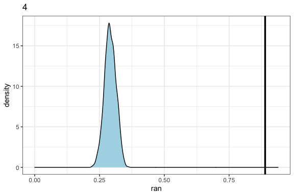

distribution.plot(netfacs.data = angry.face)$"9"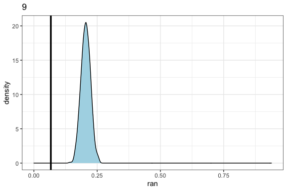

This already gives us an important insight into the structure of facial expressions, by clarifying how strongly certain facial muscles are connected to specific contexts. What we can do now is look at higher-order combinations of Action Units. Let’s look at combinations of 3 Action Units. As there are many combinations that only occur once or twice, and these are probably not very important, let’s set the minimum count that we consider meaningful to 5. It is important to note that, given the large number of possible higher-order combinations (e.g., 20 elements create over 1100 combinations of 3, almost 5000 combinations of 4 etc), most of these will not have meaningful information unless the data set is quite large.

# extract information for three-element-combinations in angry faces

anger.aus3 <- netfacs_extract(
  netfacs.data = angry.face,
  combination.size = 3, # only looking at combinations with 3 elements (here, Action Units)
  min.count = 5, # minimum number of times that the combination should occur
  min.prob = 0, # minimum observed probability of the combination
  min.specificity = 0, # minimum specificity of the combination
  significance = 0.01
) # significance level we are interested in

Results of netfacs_extract function for combinations of three elements

Here, we see that for example combination AU4_17_23 appears 28 times (62% of all angry faces), which is 44 times more than we would have expected. Many of the combinations only occur in the angry condition, and they get assigned an ‘increased probability’ value of NA. That many of these higher-order combinations contain very similar combinations (e.g. AU4_17_23 and AU4_17_24) can mean two things: either, they are significant because all these elements declare anger and they are combined randomly; or they are all part of one standard higher-order combination (e.g. AU4_17_23_24) that occurs over and over again. By looking at the different levels (3rd order, 4th order etc), we can resolve this question.

Element specificity

One question that is of relevance in this context is which element actually contributes to our decoding of the message that the other one is trying to send. For example, AU1 and AU2 will both appear on their own, but also as AU1+2, AU1+2+5, AU1+2+5+26 etc. The question is whether the elements actually add information about the condition: If I remove AU1 from AU1+2+5+26, does the resulting combination still convey the same message? We do this through the specificity measure (i.e., strength association of the element with the condition in question): the function ‘element.specificity’ goes through all combinations that contain an element and calculates the mean specificity with and without the element. The result tells us which Action Units actually add the information ‘angry!’ and which ones potentially just appear as part of combinations:

specificity <- element.specificity(netfacs.data = angry.face)

Here, we see that even though AU5 is pretty rare, as it only occurred 6 times, and is in itself not very specific to the context of anger (only 5% of all events containing AU5 occur in anger), adding AU5 to other combinations makes them ‘angry’: the specificity increases by 35%. Combinations that would usually be relatively neutral (for example, wrinkling your forehead) look really angry if you add some eye flashing. Thus, AU5 on itself is not a sign of anger, but when added to other combinations it might have a different function. A smile (AU12) actually decreases the likelihood that a combination is ‘angry’ (specificity increase = -0.09). The specificity increase is available for the first level (single elements) and second level (dyads of elements).

Results of the specificity increase in combinations due to to inclusion of each element

To understand the importance of any element in our communication system, we should look for the ones that combine two aspects: they should be common in the context (i.e., high probability), but they should also be limited to that context (i.e., high specificity). We will come back to that idea when talking about the overlap networks below.

Conditional probability between elements

The previous sections all dealt with the unconditional probability of two elements occurring together; for example, we wanted to know whether Action Units 1 and 2 occur together more often than expected. However, these two elements will sometimes occur together and sometimes on their own, and this might be important from a communication point of view: for example, if AU1 is always active when AU2 is there, and vice versa, it is reasonable to assume that these two elements are actually used as one functional unit. These two elements would have respective conditional probabilities of 1, or close to it. Alternatively, two elements could have conditional probabilities of 0; this could indicate that sender use either one or the other. For example, in facial expressions, AU26 (jaw drop) and AU27 (mouth stretch) denote different levels of opening the mouth, and they can never happen at the same time, which is a relevant aspect of the structure of the FACS. The conditional probabilities of two elements can be highly asymmetric: AU2 can always be associated with AU1, but AU1 can be more common and happen outside of this combination. This case will usually indicate that one element is either way more common than the other, or that the second one functions to change the meaning of the other. For example, consonants in English, when spoken, include a vowel, so the conditional probability of hearing the vowel when the consonant is used is 1; however, the same vowel is shared between many consonants. The last alternative is the the two elements are not related to each other and randomly co-occur across events.

In NetFACS, we can get information on the conditional probabilities using the ‘network.conditional’ function, which also gives us a network representation (discussed below). If we are simply interested in the conditional probabilities themselves, we use the following function:

conditional.probs <- network.conditional(
  netfacs.data = angry.face,
  min.prob = 0,
  min.count = 5,
  ignore.element = NULL
)

Conditional probabilities for a subset of dyadic combinations

The above table shows us the two elements (e.g., 5 an 23), how often they occur together (‘count’), the probability of each of them to occur across events P(A) and P(B); their unconditional probability to occur together P(A+B), and the probability of A occurring when B is also present. So for the AU 5 and 23, AU23 is much more common in angry faces (80% of videos) than AU5 (13% of videos). They also occur both together in 13% of cases, which means that in all cases where AU5 was observed, AU23 was also observed, but only 17% of events that have AU23 also have AU5 present. In this case, it appears as if AU5 is an ‘addition’ to AU23 or facial expressions including AU23. If we look at AU17 and AU23, they appear to be part of a fixed expression: their conditional probabilities are around 80% each way, indicating that they both occur together most of the time. Below, we will also show what the network visualisation of this function looks like.

\newpage

Networks

Now that we have our information about the probabilities of different elements and conditions extracted, we can start looking at different networks that potentially contain information about our Action Units that we rarely consider. There are different networks here that are of interest: first, we can make a bipartite network that shows us how different conditions are linked and which Action Units are specific to certain context. To a have high information value, we would expect an Action Unit to have high specificity in one context and that context only. Second, we can use networks to visualise the connections between Action Units. Third, we can use network metrics to identify central Action Units in a condition, and understand the network as a whole better.

Overlap networks

Let’s start with the bipartite overlap network: we can visualise which conditions (in our case, emotions), share Action Units. To make the process easier, there is a ‘netfacs_multiple’ function that runs the netfacs function for all levels of a condition against all others.

multi.facs <- netfacs_multiple(
  data = au.data,
  condition = au.info$emotion,
  ran.trials = 1000,
  combination.size = 2,
  use_parallel = TRUE
)

Now we can make a network where each condition is a node, and they are connected through the Action Units. We only consider Action Units that occur at least 3 times in the condition. Let’s also remove Action Unit 25 because it can be created by different muscles and is therefore ambiguous. The overlap.network function creates different graphs for different questions: the ‘specificity’ graph shows the conditional probability that we are in a condition given that we observe the element; the ‘occurrence’ graph shows the conditional probability to observe an element in a given context:

overlap.net <- overlap.network(
  netfacs.list = multi.facs,
  min.prob = 0, # minimum probability of a connection to be included
  min.count = 3, # minimum count of co-occurrences for a connection to be included
  significance = 0.01, # significance level for combinations to be considered
  clusters = FALSE, # should the bipartite network be clustered
  plot.bubbles = TRUE,
)

plot(overlap.net$specificity)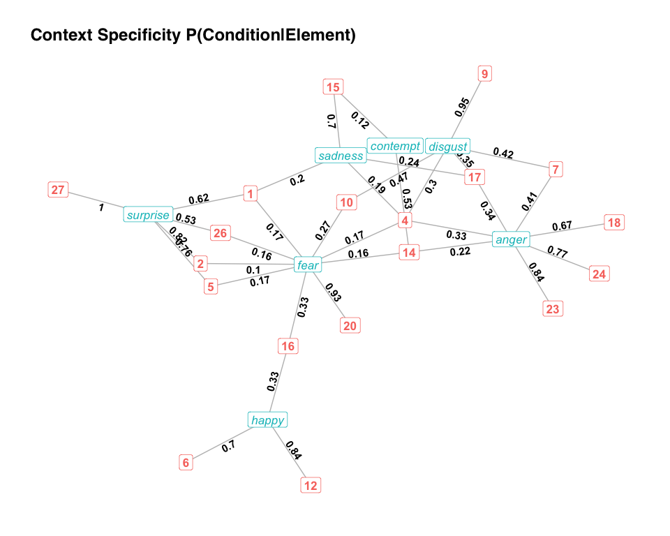

plot(overlap.net$occurrence)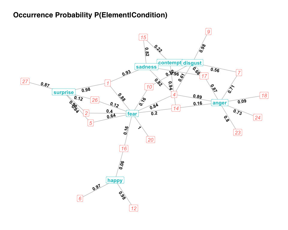

Now, we have an easy way to understand our FACS data: Above we see how specific an AU is to a condition. 84% of all AU12 happen in happy faces; while all AU27 happen in surprised faces. AU4 is shared between multiple conditions without being specific to any of them. Below, we have the occurrence data: AU6 and AU12 occur in almost all ‘happy’ faces, but AU16 is rare (P = 0.06). AU15 occurs in 82% of sad faces, and 22% of contemptuous faces. The underlying data are stored in the overlap.network object as well, in case the network is overwhelmingly full and hard to understand. With the ‘clusters’ parameter, we could explore whether these results create clearly separated clusters using the igraph ‘fast and greedy’ clustering algorithm.

Conditional probability networks

Earlier, we explored conditional probability, but we did not yet look at the output graph, which can help us illuminate our data even more. We restrict connections to those that are at least 0.5 to make things easier to understand.

conditional.probs <- network.conditional(
  netfacs.data = angry.face,
  min.prob = 0.5,
  min.count = 5,
  ignore.element = NULL,
  plot.bubbles = TRUE
)

# plot conditional probabilities
conditional.probs$plot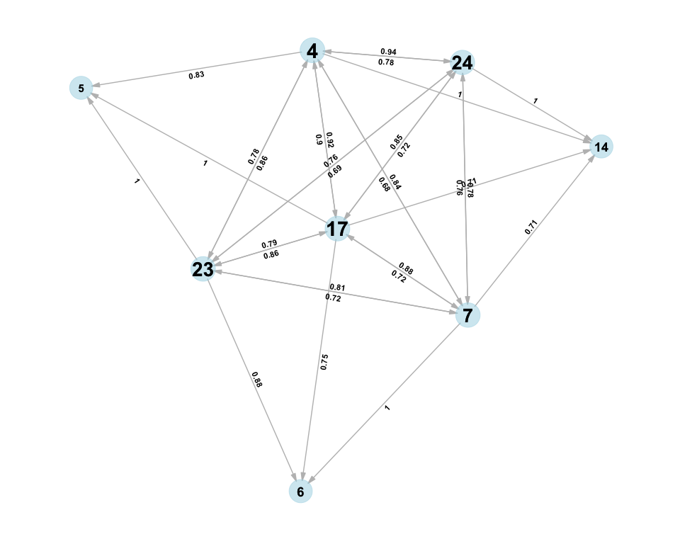

Here, we see a visual representation of the angry face and how the AUs are linked: for example, AU4, 17, 23, and 24 are bigger than the others, indicating that they are more common. Accordingly, AU17 and AU23 happen almost every time when AU6 is active, but AU6 does not happen above our threshold of 0.5 for cases with those AUs active. The common AUs, on the other hand (e.g., AU4 and 23) have reciprocal conditional probability: in the majority of cases when one is active, the other one is also active.

Network visualisation

To do all the following calculations, we extract the netfacs object and turn it into a network with specific properties. Here goes:

angry.net <- netfacs.network(
  netfacs.data = angry.face,
  link = "unweighted", # edges are linked for significant results only
  significance = 0.01,
  min.count = 3, # remove rare elements as they might be random variation
  min.prob = 0
)

Now we have our angry.net, which is an ‘igraph’ object. ‘igraph’ is the most commonly used package for network analysis in R, so now we can use all the functions that have been developed for plotting and analysing networks.

Let’s plot our network for angry faces.

network.plot(
  netfacs.graph = angry.net,
  title = "angry network",
  clusters = FALSE,
  plot.bubbles = TRUE,
  hide.unconnected = TRUE
)

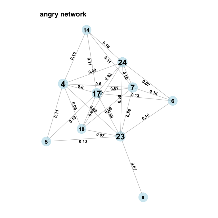
This looks like a pretty tight cluster of some Action Units that tend to occur together. AU5 and AU6 are not significantly more common in this context than expected, but occur in combination with other AUs more than expected (that’s why they are smaller). This is again relatively different from the other networks: we can apply the netfacs.network function across our conditions to get a visual representation of how networks differ:

multi.net <- multiple.netfacs.network(
  netfacs.list = multi.facs,
  link = "weighted", # network contains edges where significantly connected
  significance = 0.01,
  min.count = 3, # again remove rare connections
  min.prob = 0
)

multiple.network.plot(netfacs.graphs = multi.net)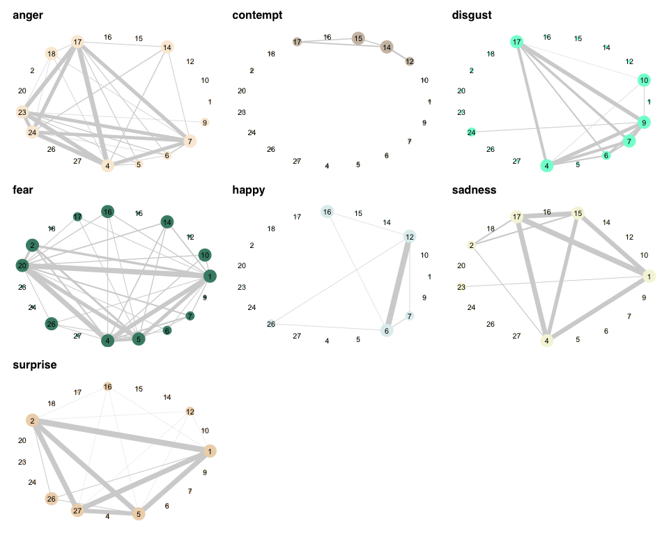

Here, we can see that the network for anger actually looks pretty complex compared to the other networks: in Contempt, only the combination of AU12 and 14 occurs more often than expected. Also, not all dyads in Anger are connected, indicating that they do not always all occur together. This is very different in Surprise, for example, where all significant AUs are also significantly more likely to co-occur.

One interesting aspect of network analysis is that we might be able to move away from our posed facial expressions and detect unknown underlying patterns. For example, if we would not know which emotion was posed, would we be able to analytically detect the basic emotions because specific Action Units cluster with each other? Let’s create a network based on all data.

all.face <-
  netfacs(
    data = au.data,
    condition = NULL,
    ran.trials = 1000,
    combination.size = 2,
    use_parallel = TRUE
  )
all.net <-
  netfacs.network(netfacs.data = all.face,
                  min.count = 3,
                  link = "unweighted")

In this network, dyadic connections between Action Units mean that they occur more often together than would be expected given their own likelihood and the number of elements per event. When plotting this network, we can say ‘clusters = TRUE’. In that case, ‘igraph’ has a community detection algorithm (groups of AUs that form clusters).

network.plot(
  netfacs.graph = all.net,
  title = "all network with clusters",
  clusters = TRUE,
  plot.bubbles = TRUE
)

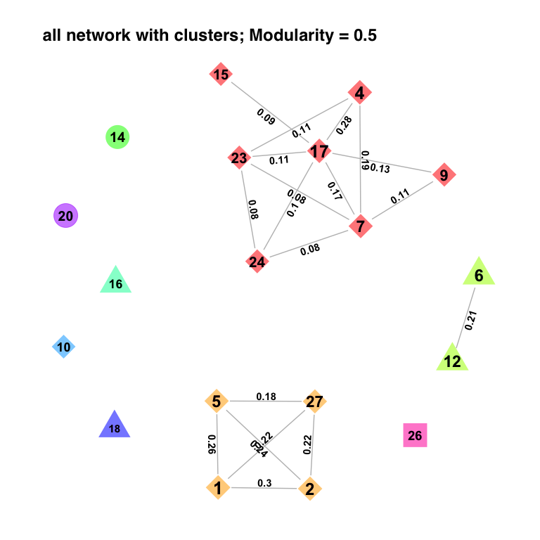
Modularity is high (0.50; above 0.3 is high). This means that there are clear clusters (AUs that are connected with each other, but not others). First, some AUs just drop out because they do not connect with any of the others (AU10, 14, 16, 18, 26). Then we have a ‘happy’ network (AU6 and AU12), a ‘surprise’ and ‘fear’ network (AU1, 2, 5, 20, 27). Anger, Sadness, and Disgust all overlap in their use of AU4 and 17, which are also the most central AUs of the remaining cluster. AU14, which is the most common AU in contempt, does not fall into either of these clusters. Given the small size of this data set, even without previous knowledge of where the emotions fall, we could assume that there are at least three distinct clusters in the data.

Network parameters

While making graphs is nice, having our FACS data as networks also allows us to calculate the centrality and importance of specific elements in the network. Again, an Action Unit that conclusively describes a specific emotion should be highly central in that network, but not at all central in any other. There are a number of different centrality measures, and one can extract them all at once.

net.sum <- network.summary(angry.net)

Network centrality measures for angry faces

The different network measures capture different aspects of centrality.

• strength: how many connections does the AU have
• eigenvector: high if AU is connected with a lot of AUs that also have a lot of connections
• betweenness: number of shortest connections that go through the AU; does it connect otherwise unconnected elements?
• transitivity: how many triads is the element in (triad == all three elements are connected)
• hub_score: similar to eigenvector
• page_rank: calculates the influence an element has over all it’s neighbours
• modularity: if modularity is high, the element clearly clusters with other elements
• community membership: elements that have the same membership cluster with each other
• community.value: if this is above 0.3, then there are clearly distinct clusters in this data set

While these centrality measures concern the elements within a network, we can also calculate information flow etc within across a network.

net.sum.graph <- network.summary.graph(angry.net)

Network graph measures for anry faces

Here, we see that there are 19 elements, 28 connections between them, which means that 16.4% of all possible connections are filled. The graph is highly transitive (== if A and B are connected and A and C are connected, B and C are also connected), so the dyadic connections probably arise out of higher-order combinations. The diameter is the ‘furthest’ connection. The degree centralisation is the mean degree/strength of all elements. Mean distance is the mean number of ‘steps’ to get from one element to the next in the network.

Let’s see what happens if we do this across the different emotions.

xx <- lapply(multi.net, function(x) {
  network.summary.graph(x)
})
xx <- do.call(rbind, xx)
xx <- cbind(emotion = names(multi.net), xx)

Network graph measures for all faces

We see that the density of the different emotion networks differs considerably, but they all have pretty low density (mainly because they all rely on a small set of AUs). Fear and Anger seem to involve more AUs than the others. Some (Anger, Surprise, Disgust) are pretty transitive (AUs all usually appear together), while some (Fear, Happy) are less transitive (indicating that they have different configurations).

Combination sizes

One question that might be of interest when we talk about complexity could be whether the number of elements is larger than expected in a context: for example, it might be that happy faces usually use fewer elements than angry faces because there is less information necessary to transmit the message. The ‘netfacs’ function also pops out the observed probabilities that events consist of 1, 2, 3 … elements, and this is tested against the null distribution.

event.size.angry <- angry.face$event.size.information
size.plot <- event.size.plot(netfacs.data = angry.face)

Combination sizes of facial expressions in the angry condition

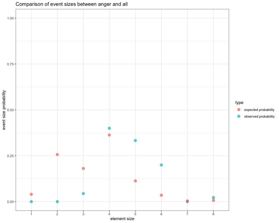
What the table and plot show us is that angry faces are actually quite complex, compared to the other emotions: events containing 0-3 Action Units are basically absent; combinations of 5, 6 and 8 Action Units are significantly more common than expected. Combinations of 4 Action Units are common (making up more than a third of cases), but this is within the range of combination sizes for all emotions.

If we do the same for happy faces, we see a very different pattern

Combination sizes of happy expressions in the angry condition

In happy faces, combinations of 2 elements are by far the most likely, while all other combination sizes occur less than expected.

Entropy

There is surprisingly little work on the information contained in facial expressions, even though this would be a great way to measure complexity. One way to quantify the amount of information in a system is by looking at how informative each observed case is. The idea is that, if in a condition, all events are exactly the same, this condition is very easily predicted and adding cases will add little information. In contrast, if under the condition, all observed events are different, then each new case that is observed adds information about the condition. This is the underlying idea of entropy measures: Entropy is maximal in entirely random systems. Entropy is minimal in perfectly ordered systems. There is potentially an insane amount of information in FACS data: for example, 30 elements can be combined in around 8 billion different ways. We know this is not the case, so there is clearly order and rules in the system.

There are two ways of looking at entropy: one is to determine how much entropy there is in a system as a whole, compared to what we would predict if the system was entirely random. In an ordered system, few of the possible options should be selected, the difference between observed and random entropy should be large, telling us that it would be easy to predict what happens. In a complex system, lots of possible options are selected, the observed entropy approaches the random entropy, so predicting each new facial expression is harder. So, the first entropy measure gives the ratio between observed overall entropy and predicted overall entropy under random conditions.

xx <- lapply(multi.facs, function(x) {
  entropy.overall(x)
})
xx <- do.call(rbind, xx)
xx <- cbind(emotion = names(multi.facs), xx)

Ratios between expected and observed entropies in different emotions

Here, we see that the different emotions differ in terms of their entropy ratio (ratios close to 0 mean order, ratios close to 1 mean chaos). As we can see, happy and surprised faces, which are both made up of mainly one expression, are very predictable. Fear, on the other hand, where no two expressions are exactly the same, is highly chaotic. With increasing sample size, this would probably change, but the difference between contexts is still quite robust.

Exporting networks

While the NetFACS package provides convenience functions to visualize networks, some users may prefer to explore their networks using other software such as gephi. It is easy to convert networks into a matrix or table by using igraph’s conversion functions, which can then be saved as a CSV file and imported into other software. For example:

# create an edge table
anger.tab <- igraph::as_data_frame(multi.net$anger)

# create an adjacency matrix
anger.adj.mat <- as.matrix(igraph::as_adjacency_matrix(multi.net$anger))

# save as CSV file
# write.csv(anger.tab, "anger_net_tab.csv")
# write.csv(anger.adj.mat, "adj_net_mat.csv")