![]()
![]()
Table of contents: Overview - Installation - Usage - File types - Contact
RaMS is a lightweight package that provides rapid and tidy access to mass-spectrometry data. This package is lightweight because it’s built from the ground up rather than relying on an extensive network of external libraries. No Rcpp, no Bioconductor, no long load times and strange startup warnings. Just XML parsing provided by xml2 and data handling provided by data.table. Access is rapid because an absolute minimum of data processing occurs. Unlike other packages, RaMS makes no assumptions about what you’d like to do with the data and is simply providing access to the encoded information in an intuitive and R-friendly way. Finally, the access is tidy in the philosophy of tidy data. Tidy data neatly resolves the ragged arrays that mass spectrometers produce and plays nicely with other tidy data packages.
To install the stable version on CRAN:
To install the current development version:
Finally, load RaMS like every other package:
There’s only one main function in RaMS: the aptly named grabMSdata. This function accepts the names of mass-spectrometry files as well as the data you’d like to extract (e.g. MS1, MS2, BPC, etc.) and produces a list of data tables. Each table is intuitively named within the list and formatted tidily:
msdata_dir <- system.file("extdata", package = "RaMS")
msdata_files <- list.files(msdata_dir, pattern = "mzML", full.names=TRUE)
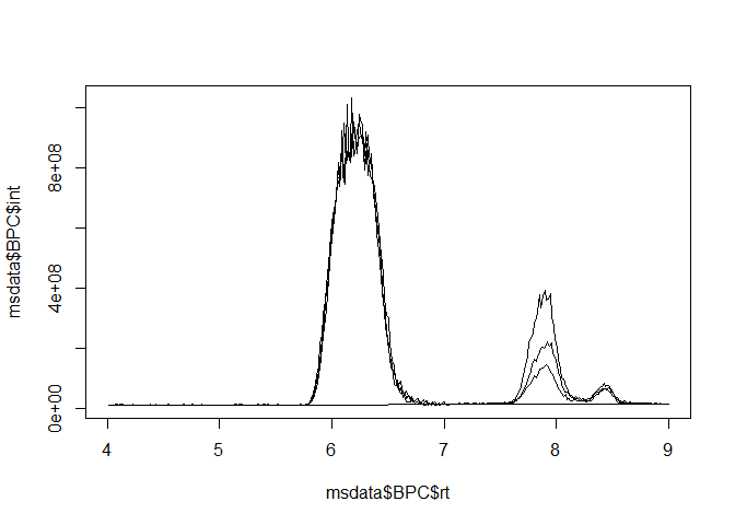
msdata <- grabMSdata(files = msdata_files[2:4], grab_what = c("BPC", "MS1"))Base peak chromatograms (BPCs) and total ion chromatograms (TICs) have three columns, making them super-simple to plot with either base R or the popular ggplot2 library:
| rt | int | filename |
|---|---|---|
| 4.009000 | 11141859 | LB12HL_AB.mzML.gz |
| 4.024533 | 9982309 | LB12HL_AB.mzML.gz |
| 4.040133 | 10653922 | LB12HL_AB.mzML.gz |
library(ggplot2)
ggplot(msdata$BPC) + geom_line(aes(x = rt, y=int, color=filename)) +
  facet_wrap(~filename, scales = "free_y", ncol = 1) +
  labs(x="Retention time (min)", y="Intensity", color="File name: ") +
  theme(legend.position="top")
MS1 data includes an additional dimension, the m/z of each ion measured, and has multiple entries per retention time:
| rt | mz | int | filename |
|---|---|---|---|
| 4.009 | 104.0710 | 1297755.00 | LB12HL_AB.mzML.gz |
| 4.009 | 104.1075 | 140668.12 | LB12HL_AB.mzML.gz |
| 4.009 | 112.0509 | 67452.86 | LB12HL_AB.mzML.gz |
This tidy format means that it plays nicely with other tidy data packages. Here, we use [data.table] and a few other tidyverse packages to compare a molecule’s 13C and 15N peak areas to that of the base peak, giving us some clue as to its molecular formula.
library(data.table)
library(tidyverse)

M <- 118.0865
M_13C <- M + 1.003355
M_15N <- M + 0.997035

iso_data <- imap_dfr(lst(M, M_13C, M_15N), function(mass, isotope){
  peak_data <- msdata$MS1[mz%between%pmppm(mass) & rt%between%c(7.6, 8.2)]
  cbind(peak_data, isotope)
})

iso_data %>%
  group_by(filename, isotope) %>%
  summarise(area=sum(int)) %>%
  pivot_wider(names_from = isotope, values_from = area) %>%
  mutate(ratio_13C_12C = M_13C/M) %>%
  mutate(ratio_15N_14N = M_15N/M) %>%
  select(filename, contains("ratio")) %>%
  pivot_longer(cols = contains("ratio"), names_to = "isotope") %>%
  group_by(isotope) %>%
  summarize(avg_ratio = mean(value), sd_ratio = sd(value), .groups="drop") %>%
  mutate(isotope=str_extract(isotope, "(?<=_).*(?=_)")) %>%
knitr::kable()| isotope | avg_ratio | sd_ratio |
|---|---|---|
| 13C | 0.0543929 | 0.0006015 |
| 15N | 0.0033375 | 0.0001846 |
With natural abundances for 13C and 15N of 1.11% and 0.36%, respectively, we can conclude that this molecule likely has five carbons and a single nitrogen.
Of course, it’s always a good idea to plot the peaks and perform a manual check of data quality:
ggplot(iso_data) +
  geom_line(aes(x=rt, y=int, color=filename)) +
  facet_wrap(~isotope, scales = "free_y", ncol = 1)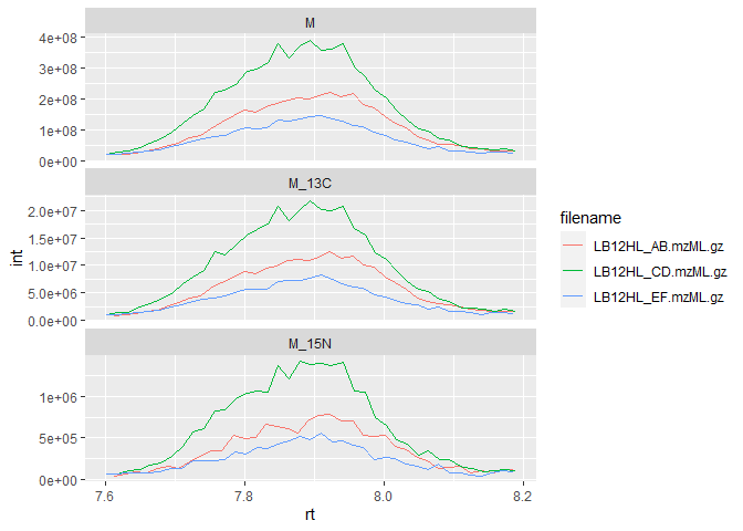
DDA (fragmentation) data can also be extracted, allowing rapid and intuitive searches for fragments or neutral losses:
For example, we may be interested in the major fragments of a specific molecule:
msdata$MS2[premz%between%pmppm(118.0865) & int>mean(int)] %>%
  plot(int~fragmz, type="h", data=., ylab="Intensity", xlab="Fragment m/z")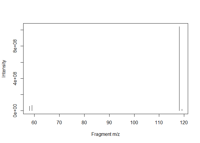
Or want to search for a specific neutral loss:
msdata$MS2[, neutral_loss:=premz-fragmz] %>%
  filter(neutral_loss%between%pmppm(60.02064, 5)) %>%
head() %>% knitr::kable()| rt | premz | fragmz | int | voltage | filename | neutral_loss |
|---|---|---|---|---|---|---|
| 4.182333 | 118.0864 | 58.06590 | 390179.500 | 35 | DDApos_2.mzML.gz | 60.02055 |
| 4.276100 | 116.0709 | 56.05036 | 1093.988 | 35 | DDApos_2.mzML.gz | 60.02050 |
| 4.521367 | 118.0864 | 58.06589 | 343084.000 | 35 | DDApos_2.mzML.gz | 60.02056 |
| 4.649867 | 170.0810 | 110.06034 | 4792.479 | 35 | DDApos_2.mzML.gz | 60.02070 |
| 4.857983 | 118.0865 | 58.06590 | 314075.312 | 35 | DDApos_2.mzML.gz | 60.02057 |
| 5.195617 | 118.0865 | 58.06590 | 282611.688 | 35 | DDApos_2.mzML.gz | 60.02057 |
RaMS is currently limited to the modern mzML data format and the slightly older mzXML format. Tools to convert data from other formats are available through Proteowizard’s msconvert tool. Data can, however, be gzip compressed (file ending .gz) and this compression actually speeds up data retrieval significantly as well as reducing file sizes.
Currently, RaMS also handles only MS1 and MS2 data. This should be easy enough to expand in the future, but right now I haven’t observed a demonstrated need for higher fragmentation level data collection.
Additionally, note that files can be streamed from the internet directly if a URL is provided to grabMSdata, although this will usually take longer than reading a file from disk:
## Not run:
# Find a file with a web browser:
browseURL("https://www.ebi.ac.uk/metabolights/MTBLS703/files")

# Copy link address by right-clicking "download" button:
sample_url <- paste0("https://www.ebi.ac.uk/metabolights/ws/studies/MTBLS703/",
                     "download/acefcd61-a634-4f35-9c3c-c572ade5acf3?file=",
                     "161024_Smp_LB12HL_AB_pos.mzXML")
msdata <- grabMSdata(sample_url, grab_what="everything", verbosity=2)
msdata$metadataFeel free to submit questions, bugs, or feature requests on the GitHub Issues page.
README last built on 2021-03-17