The StrucDiv package provides methods to quantify
spatial structural diversity, hereafter structural diversity, in raster
data. Raster data means data in gridded field format. The methods
consider the spatial arrangement of pixels as pairs, based on Haralick,
Shanmugam, and Dinstein (1973). Pixels are considered as pairs at
user-specified distances and angles. Distance refers to the distance
between the two pixels that are considered a pair. Angle refers to the
angle at which two pixels are considered a pair. Angles can be
horizontal or vertical direction, or the diagonals at 45° or 135°. the
direction-invariant version considers all angles at the same time. The
frequencies of pixel pair occurrences are normalized by the total number
of pixel pairs, which returns the gray level co-occurrence matrix
(GLCM). The total number of pixel pairs depends on the extent of the
area under consideration, i.e. on the spatial scale. the spatial scale
is defined by the window side length (WSL) of a moving window. In each
GLCM, pixel values can be replaced with ranks. Diversity metrics are
calculated on every element of the GLCM, and their sum is assigned to
the center pixel of the moving window and represents spatial structural
diversity of the window. The output map is called a ‘structural
diversity map.’ Diversity metrics include common second-order texture
metrics: contrast, dissimilarity, homogeneity and entropy (i.e. Shannon
entropy). Additionally, structural diversity entropy includes a
difference weight δ ∈ {0, 1, 2}, which weighs the difference
between pixel values vi and vj,
either by absolute, or by squared differences. When δ = 0,
structural diversity entropy corresponds to Shannon entropy.
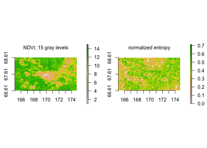
Additionally, normalized entropy is available. Normalized entropy is
Shannon entropy normalized over maximum entropy, which depends on the
spatial scale. These methods can be applied to any continuous data in
raster format, and also to categorical data if categories are numbered
in a meaningful way, or if entropy or normalized entropy are used. For
entropy, normalized entropy, and homogeneity, high numbers of gray
levels lead to structureless diversity maps. With these methods,
structural diversity features can be detected. Structural diversity
features have also been called latent landscape features.
You can install the released version of StrucDiv from CRAN with:
install.packages("StrucDiv")Calculate normalized entropy on Normalized Difference Vegetation Index (NDVI) data, which was binned to 15 gray levels (see data documentation). We define the size of the moving window with WSL three, and we consider distance one between pixels (direct neighbors), and all four possible directions in which pixels can be considered as pairs.
entNorm <- StrucDiv(ndvi.15gl, wsl = 5, dist = 1, angle = "all", fun = entropyNorm, na.handling = na.pass)