![]()
![]()
The USgas package provides an overview of demand for natural gas in the US in a time-series format. That includes the following datasets:
us_total - The US annual natural gas consumption by state-level between 1997 and 2019, and aggregate level between 1949 and 2019us_monthly - The monthly demand for natural gas in the US between 2001 and 2020us_residential - The US monthly natural gas residential consumption by state and aggregate level between 1989 and 2020Data source: The US Energy Information Administration API
More information about the package datasets available on this vignette.
You can install the released version of USgas from CRAN with:
And the development version from GitHub with:
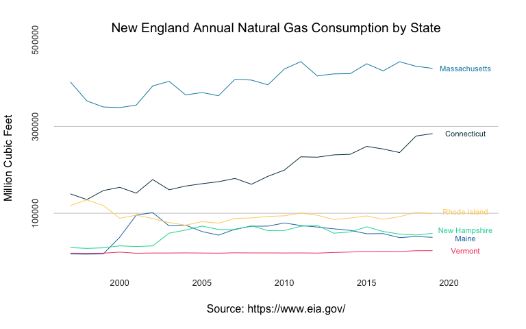
Plotting the consumption of natural gas in New England states:
data(us_total)

str(us_total)
#> 'data.frame':    1266 obs. of  3 variables:
#>  $ year : int  1997 1998 1999 2000 2001 2002 2003 2004 2005 2006 ...
#>  $ state: chr  "Alabama" "Alabama" "Alabama" "Alabama" ...
#>  $ y    : int  324158 329134 337270 353614 332693 379343 350345 382367 353156 391093 ...

head(us_total)
#>   year   state      y
#> 1 1997 Alabama 324158
#> 2 1998 Alabama 329134
#> 3 1999 Alabama 337270
#> 4 2000 Alabama 353614
#> 5 2001 Alabama 332693
#> 6 2002 Alabama 379343
Subsetting the New England states:
ne <- c("Connecticut", "Maine", "Massachusetts",
        "New Hampshire", "Rhode Island", "Vermont")
ne_gas <-  us_total[which(us_total$state %in% ne),]

ne_wide <- reshape(ne_gas, v.names = "y", idvar = "year",
                   timevar = "state", direction = "wide")
ne_wide <- ne_wide[order(ne_wide$year), ]

names(ne_wide) <- c("year",ne)

head(ne_wide)
#>     year Connecticut  Maine Massachusetts New Hampshire Rhode Island Vermont
#> 139 1997      144708   6290        402629         20848       117707    8061
#> 140 1998      131497   5716        358846         19127       130751    7735
#> 141 1999      152237   6572        344790         20313       118001    8033
#> 142 2000      159712  44779        343314         24950        88419   10426
#> 143 2001      146278  95733        349103         23398        95607    7919
#> 144 2002      177587 101536        393194         24901        87805    8367
Plotting the states series:
# Set the y and x axis ticks
at_x <- seq(from = 2000, to = 2020, by = 5)

at_y <- pretty(ne_gas$y)[c(2, 4, 6)]

# plot the first series
plot(ne_wide$year, ne_wide$Connecticut,
     type = "l",
     col = "#073b4c",
     frame.plot = FALSE,
     axes = FALSE,
     panel.first = abline(h = c(at_y), col = "grey80"),
     main = "New England Annual Natural Gas Consumption by State",
     cex.main = 1.2, font.main = 1, col.main = "black",
     xlab = "Source: https://www.eia.gov/",
     font.axis = 1, cex.lab= 1,
     ylab = "Million Cubic Feet",
     ylim = c(min(ne_gas$y, na.rm = TRUE), max(ne_gas$y, na.rm = TRUE)),
     xlim = c(min(ne_gas$year), max(ne_gas$year) + 3))

# Add the 5 other series
lines(ne_wide$year, ne_wide$Maine, col = "#1f77b4")
lines(ne_wide$year, ne_wide$Massachusetts, col = "#118ab2")
lines(ne_wide$year, ne_wide$`New Hampshire`, col = "#06d6a0")
lines(ne_wide$year, ne_wide$`Rhode Island`, col = "#ffd166")
lines(ne_wide$year, ne_wide$Vermont, col = "#ef476f")

# Add the y and x axis ticks

mtext(side =1, text = format(at_x, nsmall=0), at = at_x,
      col = "grey20", line = 1, cex = 0.8)

mtext(side =2, text = format(at_y, scientific = FALSE), at = at_y,
      col = "grey20", line = 1, cex = 0.8)

# Add text
text(max(ne_wide$year) + 2,
     tail(ne_wide$Connecticut,1),
     "Connecticut",
     col = "#073b4c",
     cex = 0.7)

text(max(ne_wide$year) + 2,
     tail(ne_wide$Maine,1) * 0.95,
     "Maine",
     col = "#1f77b4",
     cex = 0.7)

text(max(ne_wide$year) + 2,
     tail(ne_wide$Massachusetts,1),
     "Massachusetts",
     col = "#118ab2",
     cex = 0.7)

text(max(ne_wide$year) + 2,
     tail(ne_wide$`New Hampshire`,1) * 1.1,
     "New Hampshire",
     col = "#06d6a0",
     cex = 0.7)

text(max(ne_wide$year) + 2,
     tail(ne_wide$`Rhode Island`,1) * 1.05,
     "Rhode Island",
     col = "#ffd166",
     cex = 0.7)

text(max(ne_wide$year) + 2,
     tail(ne_wide$Vermont,1),
     "Vermont",
     col = "#ef476f",
     cex = 0.7)