
The adaptr package simulates adaptive clinical trials
using adaptive stopping, adaptive arm dropping and/or response-adaptive
randomisation.
The package has been developed as part of the INCEPT (Intensive Care Platform Trial) project, which is primarily supported by a grant from Sygeforsikringen “danmark”.
The full package documentation is available as a stand-alone website at inceptdk.github.io/adaptr.
# The easiest way is to install from CRAN directly
install.packages("adaptr")

# But you can also get the newest version from GitHub (requires the remotes package)
# install.packages("remotes")
remotes::install_github("INCEPTdk/adaptr")The basic functionality of adaptr is illustrated
below.
First, load the library and setup a trial specification using the
general setup_trial() function, or one of the special case
functions, setup_trial_binom() (used in the example) or
setup_trial_norm().
library(adaptr)
#> Loading adaptr package (version 1.1.0).
#> See 'help("adaptr")' or 'vignette("Overview", "adaptr")' for help.
#> Further information available on https://inceptdk.github.io/adaptr/.

# Setup a trial using a binary, binomially distributed, undesirable outcome
binom_trial <- setup_trial_binom(
  arms = c("Arm A", "Arm B", "Arm C"),
  true_ys = c(0.25, 0.20, 0.30),
  min_probs = rep(0.15, 3), # Minimum allocation of 15% in all arms
  data_looks = seq(from = 300, to = 2000, by = 100),
  # Stop for equivalence at > 90% probability of differences < 5 %-points
  equivalence_prob = 0.9,
  equivalence_diff = 0.05,
  soften_power = 0.5 # Soften allocation ratios
)

# Print trial specification
print(binom_trial, prob_digits = 3)
#> Trial specification: generic binomially distributed outcome trial
#> * Undesirable outcome
#> * No common control arm
#> * Best arm: Arm B
#>
#> Arms, true outcomes, starting allocation probabilities
#> and allocation probability limits:
#>   arms true_ys start_probs fixed_probs min_probs max_probs
#>  Arm A    0.25       0.333          NA      0.15        NA
#>  Arm B    0.20       0.333          NA      0.15        NA
#>  Arm C    0.30       0.333          NA      0.15        NA
#>
#> Maximum sample size: 2000
#> Maximum number of data looks: 18
#> Planned data looks after:  300, 400, 500, 600, 700, 800, 900, 1000, 1100, 1200, 1300, 1400, 1500, 1600, 1700, 1800, 1900, 2000 patients
#>
#> Superiority threshold: 0.99
#> Inferiority threshold: 0.01
#> Equivalence threshold: 0.9 (no common control)
#> Absolute equivalence difference: 0.05
#> No futility threshold (not relevant - no common control)
#> Soften power for all analyses: 0.5
Simulate a single trial using a reproducible random seed:
trial_res <- run_trial(binom_trial, seed = 12345)
print(trial_res, digits = 3)
#> Single simulation result: generic binomially distributed outcome trial
#> * Undesirable outcome
#> * No common control arm
#>
#> Final status: inconclusive, stopped at maximum sample size
#> Final/maximum allowed sample sizes: 2000/2000 (100.0%)
#>
#> Final trial results:
#>   arms true_ys sum_ys  ns raw_ests post_ests post_errs lo_cri hi_cri
#>  Arm A    0.25    180 742    0.243     0.243    0.0159  0.213  0.275
#>  Arm B    0.20    178 841    0.212     0.212    0.0141  0.185  0.241
#>  Arm C    0.30    113 417    0.271     0.271    0.0215  0.230  0.316
#>  final_status status_look status_probs final_alloc
#>        active          NA           NA       0.194
#>        active          NA           NA       0.656
#>      inferior        2000        0.007       0.150
#>
#> Simulation details:
#> * Random seed: 12345
#> * Credible interval width: 95%
#> * Number of posterior draws: 5000
#> * Posterior estimation method: medians with MAD-SDs
Simulate multiple trials using a reproducible random seed:
# Simulate multiple trials - only 10 simulations for speed in the example
trial_res_mult <- run_trials(binom_trial, n_rep = 10, base_seed = 67890)

# Extract results in a tidy data.frame (1 simulation per row)
# See function documentation for details, including on arm selection in trials
# not ending with a superior arm
extr_res <- extract_results(trial_res_mult)
head(extr_res)
#>   sim final_n sum_ys  ratio_ys final_status superior_arm selected_arm
#> 1   1    2000    415 0.2075000          max         <NA>         <NA>
#> 2   2     600    139 0.2316667  superiority        Arm B        Arm B
#> 3   3    1000    237 0.2370000  superiority        Arm B        Arm B
#> 4   4     900    209 0.2322222  equivalence         <NA>         <NA>
#> 5   5    2000    441 0.2205000  superiority        Arm B        Arm B
#> 6   6    1900    431 0.2268421  superiority        Arm B        Arm B
#>         sq_err sq_err_te
#> 1           NA        NA
#> 2 7.853843e-04        NA
#> 3 4.190319e-05        NA
#> 4           NA        NA
#> 5 3.422824e-06        NA
#> 6 4.852161e-05        NA

# Summarise trial results
# See function documentation for details, including on arm selection in trials
# not ending with a superior arm
res_sum <- summary(trial_res_mult)
print(res_sum, digits = 1)
#> Multiple simulation results: generic binomially distributed outcome trial
#> * Undesirable outcome
#> * Number of simulations: 10
#> * Number of simulations summarised: 10 (all trials)
#> * No common control arm
#> * Selection strategy: no selection if no superior arm
#> * Treatment effect compared to: no comparison
#>
#> Performance metrics (using posterior estimates):
#> * Sample sizes: mean 1470.0 (SD: 559.9) | median 1550.0 (IQR: 1025.0 to 2000.0)
#> * Total summarised outcomes: mean 323.3 (SD: 110.6) | median 340.0 (IQR: 242.0 to 421.8)
#> * Total summarised outcome rates: mean 0.224 (SD: 0.013) | median 0.229 (IQR: 0.214 to 0.233)
#> * Conclusive: 70.0%
#> * Superiority: 50.0%
#> * Equivalence: 20.0%
#> * Futility: 0.0% [not assessed]
#> * Inconclusive at max sample size: 30.0%
#> * Selection probabilities: Arm A: 0.0% | Arm B: 50.0% | Arm C: 0.0% | None: 50.0%
#> * RMSE: 0.01330
#> * RMSE treatment effect: not estimated
#> * Ideal design percentage: 100.0%
#>
#> Simulation details:
#> * Simulation time: 0.388 secs
#> * Base random seed: 67890
#> * Credible interval width: 95%
#> * Number of posterior draws: 5000
#> * Estimation method: posterior medians with MAD-SDs
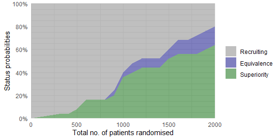
Plot trial statuses or history of trial metrics over time:
# Simulate multiple trials - 25 simulations only for speed
# sparse = FALSE is required for plot_history (but not plot_status)
trial_res_mult <- run_trials(binom_trial, n_rep = 25, base_seed = 67890, sparse = FALSE)

# Plot overall trial statuses according to the total number
# of patients randomised
plot_status(trial_res_mult, x_value = "total n")
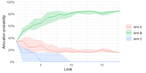
# Plot allocation probabilities at each adaptive look (requires sparse = FALSE)
plot_history(trial_res_mult)
Plotting statuses for individual trial arms and other summary metrics is possible, too.
We use the GitHub issue tracker for all bug/issue reports and proposals for enhancements.
We welcome contributions directly to the code to improve performance as well as new functionality. For the latter, please first explain and motivate it in an issue.
Changes to the code base should follow these steps:
NEWS.md file to see the formatting)main branch of
adaptrIf using the package, please consider citing it:
citation(package = "adaptr")
#>
#> To cite adaptr in publications use:
#>
#>   Granholm A, Jensen AKG, Lange T, Kaas-Hansen BS (2022). adaptr: an R
#>   package for simulating and comparing adaptive clinical trials.
#>   Journal of Open Source Software, 7(72), 4284. URL
#>   https://doi.org/10.21105/joss.04284.
#>
#> A BibTeX entry for LaTeX users is
#>
#>   @Article{,
#>     title = {{adaptr}: an R package for simulating and comparing adaptive clinical trials},
#>     author = {Anders Granholm and Aksel Karl Georg Jensen and Theis Lange and Benjamin Skov Kaas-Hansen},
#>     journal = {Journal of Open Source Software},
#>     year = {2022},
#>     volume = {7},
#>     number = {72},
#>     pages = {4284},
#>     url = {https://doi.org/10.21105/joss.04284},
#>     doi = {10.21105/joss.04284},
#>   }