
The goal of bayeslincom is to provide point estimates, standard deviations, and credible intervals for linear combinations of posterior samples. Additionally, it allows for testing against using null values using a region of practical equivalence (ROPE) approach (Kruschke and Liddell 2018).
You can install the released version of bayeslincom from CRAN with:
The development version from GitHub with:
The main function is lin_comb. The following examples show how this function can be used to test linear combinations of posterior samples in tandem with different object types.
The BBcor package provides Bayesian bootstrapped correlations and partial correlations. In the following, the test is whether the magnitude of one correlation is larger than that for a sum of two correlations. The correlations can be estimated with
library(BBcor)

# data
Y <- mtcars[, c("mpg", "wt", "hp")]

# fit model
fit_bb <- bbcor(Y, method = "spearman")

# print
fit_bb

#>           mpg         wt         hp
#> mpg  1.0000000 -0.8842590 -0.8946683
#> wt  -0.8842590  1.0000000  0.7754185
#> hp  -0.8946683  0.7754185  1.0000000
Next the hypothesis is written out. In this case
Note that each relation is multiplied by the sign. This ensures the magnitude is being compared. Next the hypothesis is tested using the lin_comb function
lin_comb(hyp,
         obj = fit_bb,
         cri_level = 0.95)

#> bayeslincom: Linear Combinations of Posterior Samples
#> ------
#> Call:
#> lin_comb.bbcor(lin_comb = lin_comb, obj = obj, cri_level = cri_level,
#>     rope = rope)
#> ------
#> Combinations:
#>  C1: -1*mpg--wt - (-1*mpg--hp + wt--hp) = 0
#> ------
#> Posterior Summary:
#>
#>    Post.mean Post.sd Cred.lb Cred.ub Pr.less Pr.greater
#> C1     -0.78   -0.78   -0.92   -0.59       1          0
#> ------
#> Note:
#> Pr.less: Posterior probability less than zero
#> Pr.greater: Posterior probability greater than zero
In this case, the sum of the relations, mpg--hp and wt--hp, are larger than the relation mpg--wt, with a posterior probability of 1.
This example also demonstrates a key contribution of bayeslincom, i.e., testing linear combinations among dependent correlations. This is the only Bayesian (and possibly in general) implementation in R.
The BGGM package (Williams and Mulder 2019; Williams et al. 2020) provides tools for Bayesian estimation and hypothesis testing within Gaussian graphical models (i.e., partial correlation networks). This package is particularly useful as it estimates the posterior distribution for a partial correlations based on ordinal (polychoric), binary (tetrachoric), or mixed data.
An ordinal network can be estimated with
library(BGGM)

# data (+ 1)
Y <- ptsd[, 1:7] + 1

# BGGM estimate
fit_bggm <- estimate(Y, type = "ordinal", iter = 100000)
Note that 1 is added to the data in order to ensure the first category is 1 when type = "ordinal".
Several combinations can then be formulated and then passed on to lin_comb. This can be done by placing strings of combinations into a vector as shown below.
# example combinations
hyps <- c("(B4--C1 + B4--C2) > (B2--C1 + B2--C2)",
"(B2--C1 + B2--C2) > (B1--C1 + B1--C2)")
# test
test <- lin_comb(hyps,
fit_bggm,
cri_level = 0.95)
test
#> bayeslincom: Linear Combinations of Posterior Samples
#> ------
#> Call:
#> lin_comb.BGGM(lin_comb = lin_comb, obj = obj, cri_level = cri_level,
#> rope = rope)
#> ------
#> Combinations:
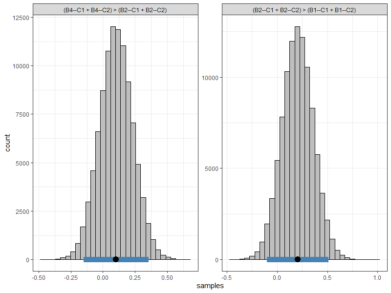
#> C1: (B4--C1 + B4--C2) > (B2--C1 + B2--C2)
#> C2: (B2--C1 + B2--C2) > (B1--C1 + B1--C2)
#> ------
#> Posterior Summary:
#>
#> Post.mean Post.sd Cred.lb Cred.ub Pr.less Pr.greater
#> C1 0.1 0.1 -0.15 0.36 0.22 0.78
#> C2 0.2 0.2 -0.10 0.51 0.10 0.90
#> ------
#> Note:
#> Pr.less: Posterior probability less than zero
#> Pr.greater: Posterior probability greater than zeroThe first combination tests whether the PTSD symptom “emotional reactivity” (B4) has a stronger relationship than the symptom “nightmares” (B2) with the cluster of nodes representing “avoidance” (C1 and C2). The second combination tests the same, except for testing for “nightmares” and “intrusive thoughts” (B1).
In addition to being the only implementation in R for testing linear combinations of (partial) correlations it is also the only implementation for testing linear combinations of polychoric and tetrachoric correlations (due to the BGGM sampling algorithms).
Objects created with lin_comb also have a plot method which returns a ggplot2 object that can further be customized, e.g.
There are a variety of R packages that provide samples from the posterior distribution. By placing the respective samples into a data.frame, bayeslincom can be used to test linear combinations. Here is an example using MCMCpack.
library(MCMCpack)

# data
Y <- mtcars

# fit model
fit_mcmc <- MCMCregress(mpg ~ vs + hp,
                        data = Y,
                        mcmc = 100000)

# data frame
samps <- as.data.frame(fit_mcmc)

# test hypothesis
test <- lin_comb(lin_comb = "vs - hp = 0",
                 obj = samps,
                 cri_level = 0.95)

# print results
fit_bayes

#> bayeslincom: Linear Combinations of Posterior Samples
#> ------
#> Call:
#> lin_comb.data.frame(lin_comb = lin_comb, obj = obj, cri_level = cri_level,
#>     rope = rope)
#> ------
#> Combinations:
#>  C1: vs - hp = 0
#> ------
#> Posterior Summary:
#>
#>    Post.mean Post.sd Cred.lb Cred.ub Pr.less Pr.greater
#> C1      2.64    2.64   -1.38    6.65    0.09       0.91
#> ------
#> Note:
#> Pr.less: Posterior probability less than zero
#> Pr.greater: Posterior probability greater than zero
Note that the hypothesis could also be written as vs = hp.
The above can also be implemented with the R package multcomp.
library(multcomp)

# fit model
fit_lm <- lm(mpg ~ vs + hp,
             data = Y)

# confidence interval
confint(
  multcomp::glht(fit_lm, linfct = "vs - hp == 0"),
  level = 0.95
  )

#>   Simultaneous Confidence Intervals
#>
#> Fit: lm(formula = mpg ~ vs + hp, data = Y)
#>
#> Quantile = 2.0452
#> 95% family-wise confidence level


#> Linear Hypotheses:
#>              Estimate lwr     upr
#> vs - hp == 0  2.6308  -1.3763  6.6378
Although the results are nearly identical, note that bayeslincom (1) provides the posterior probability of a positive and negative difference; and (2) is compatible with essentially all Rpackages for Bayesian analysis.
Testing against a null value can be done using a region of practical equivalence (ROPE) (Rouder, Haaf, and Vandekerckhove 2018; Kruschke and Liddell 2018). The ROPE approach is similar in spirit to a frequentist approach wherein a parameter value is rejected if it is not covered by a confidence interval at a particular level. The difference with the ROPE is that the null value is only rejected if there is no overlap between the credible interval and the ROPE. Conversely, the null value is only accepted if the entire credible interval is inside the ROPE.
In the following example, a model is fit using rstanarm. The difference between the coefficients for mom_iq an mom_age is tested against a null value of zero with a ROPE corresponding to [-1, 1].
library(rstanarm)

# data
Y <- kidiq

# fit model
fit_rstan <- stan_glm(kid_score ~ mom_iq + mom_age,
                      data = Y,
                      family = gaussian,
                      iter = 50000)

# data frame
samps <- as.data.frame(fit_rstan)

# test ROPE
rope <- lin_comb("mom_iq - mom_age = 0",
                  obj = samps,
                  cri_level = 0.95,
                  rope = c(-1, 1))

rope

#> bayeslincom: Linear Combinations of Posterior Samples
#> ------
#> Call:
#> lin_comb.data.frame(lin_comb = lin_comb, obj = obj, cri_level = cri_level,
#>     rope = rope)
#> ------
#> Combinations:
#>  C1: mom_iq - mom_age = 0
#> ------
#> Posterior Summary:
#>
#> ROPE: [ -1 , 1 ]
#>
#>    Post.mean Post.sd Cred.lb Cred.ub   Pr.in
#> C1      0.22    0.22   -0.44    0.88 0.98983
#> ------
#> Note:
#> Pr.in: Posterior probability in ROPE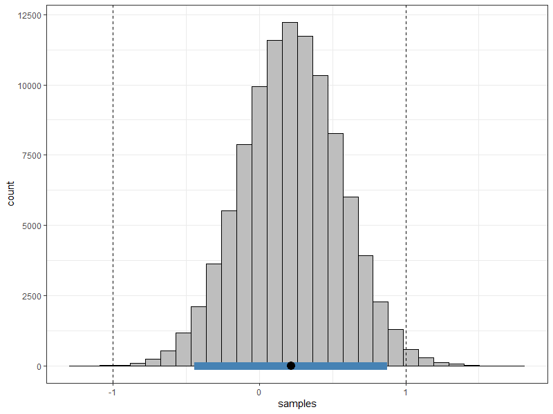
Kruschke, John K., and Torrin M. Liddell. 2018. “The Bayesian New Statistics: Hypothesis Testing, Estimation, Meta-Analysis, and Power Analysis from a Bayesian Perspective.” Psychonomic Bulletin & Review 25 (1): 178–206. https://doi.org/10.3758/s13423-016-1221-4.
Rouder, Jeffrey N., Julia M. Haaf, and Joachim Vandekerckhove. 2018. “Bayesian Inference for Psychology, Part IV: Parameter Estimation and Bayes Factors.” Psychonomic Bulletin & Review 25 (1): 102–13. https://doi.org/10.3758/s13423-017-1420-7.
Williams, Donald Ray, and Joris Mulder. 2019. “Bayesian Hypothesis Testing for Gaussian Graphical Models: Conditional Independence and Order Constraints.” Preprint. PsyArXiv. https://doi.org/10.31234/osf.io/ypxd8.
Williams, Donald R., Philippe Rast, Luis R. Pericchi, and Joris Mulder. 2020. “Comparing Gaussian Graphical Models with the Posterior Predictive Distribution and Bayesian Model Selection.” Psychological Methods. https://doi.org/10.1037/met0000254.