#> ── Attaching packages ─────────────────────────────────────── tidyverse 1.3.0 ──
#> ✓ ggplot2 3.3.5     ✓ purrr   0.3.4
#> ✓ tibble  3.1.6     ✓ dplyr   1.0.8
#> ✓ tidyr   1.2.0     ✓ stringr 1.4.0
#> ✓ readr   2.1.2     ✓ forcats 0.5.0
#> ── Conflicts ────────────────────────────────────────── tidyverse_conflicts() ──
#> x dplyr::filter() masks stats::filter()
#> x dplyr::lag()    masks stats::lag()
![]()
The goal of biogrowth is to ease the development of mathematical models to describe population growth. It includes functions for making growth predictions and for fitting growth models. The growth predictions can account for
The package includes different approaches for model fitting:
In all these cases, the package allows choosing which model parameters to estimate from the data and which ones to fix to known values.
Besides this, the package includes several additional functions to ease in the interpretation of the calculations. This includes:
The approach of biogrowth is based on the methods of predictive microbiology. Nonetheless, its equations should be applicable to other fields. It implements several mathematical models, giving the user the possibility to select among them.
The biogrowth package has been developed by researchers of the Food Microbiology Laboratory of Wageningen University and Research (the Netherlands) and the Universidad Politecnica de Cartagena (Spain).
Questions and comments can be directed to Alberto Garre (alberto.garre (at) upct.es). For bug reports, please use the GitHub page of the project.
You can install the released version of biogrowth from CRAN with:
install.packages("biogrowth")And the development version from GitHub with:
# install.packages("devtools")
devtools::install_github("albgarre/biogrowth")This is only a small sample of the functions included in the package! For a complete list, please check the package vignette.
## We will use the data on growth of Salmonella included in the package

data("growth_salmonella")

## We will fit 3 different models to the data

fit1 <- fit_growth(growth_salmonella,
                   list(primary = "Baranyi"),
                   start = c(lambda = 0, logNmax = 8, mu = .1, logN0 = 2),
                   known = c(),
                   environment = "constant",
                   )

fit2 <- fit_growth(growth_salmonella,
                   list(primary = "Baranyi"),
                   start = c(logNmax = 8, mu = .1, logN0 = 2),
                   known = c(lambda = 0),
                   environment = "constant",
                   )

fit3 <- fit_growth(growth_salmonella,
                   list(primary = "modGompertz"),
                   start = c(C = 8, mu = .1, logN0 = 2),
                   known = c(lambda = 0),
                   environment = "constant",
                   )

## We can now put them in a (preferably named) list

my_models <- list(`Baranyi` = fit1,
                  `Baranyi no lag` = fit2,
                  `Gompertz no lag` = fit3)

## And pass them to compare_growth_fits

model_comparison <- compare_growth_fits(my_models)

##  The instance of GrowthComparison has useful S3 methods

print(model_comparison)
#> Comparison between models fitted to data under isothermal conditions
#>
#> Statistical indexes arranged by AIC:
#>
#> # A tibble: 3 × 5
#>   model              AIC    df           ME   RMSE
#>   <chr>            <dbl> <int>        <dbl>  <dbl>
#> 1 Baranyi         -29.7     17  0.000000402 0.0919
#> 2 Baranyi no lag    4.49    18 -0.000000513 0.224
#> 3 Gompertz no lag   7.47    18  0.000000148 0.241
plot(model_comparison)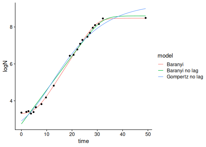
plot(model_comparison, type = 2)
plot(model_comparison, type = 3)
#> `geom_smooth()` using formula 'y ~ x'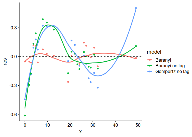
set.seed(1241)

my_model <- "Baranyi"
my_times <- seq(0, 30, length = 100)
n_sims <- 3000

pars <- tribble(
    ~par, ~mean, ~sd, ~scale,
    "logN0", 0, .2, "original",
    "mu", 2, .3, "sqrt",
    "lambda", 4, .4, "sqrt",
    "logNmax", 6, .5, "original"
)

unc_growth <- predict_growth_uncertainty(my_model, my_times, n_sims, pars)

plot(unc_growth)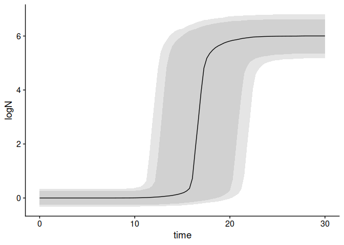
## We will use the data included in the package

data("multiple_counts")
data("multiple_conditions")

## We need to assign a model equation for each environmental factor

sec_models <- list(temperature = "CPM", pH = "CPM")

## Any model parameter (of the primary or secondary models) can be fixed

known_pars <- list(Nmax = 1e8, N0 = 1e0, Q0 = 1e-3,
                   temperature_n = 2, temperature_xmin = 20,
                   temperature_xmax = 35,
                   pH_n = 2, pH_xmin = 5.5, pH_xmax = 7.5, pH_xopt = 6.5)

## The rest, need initial guesses

my_start <- list(mu_opt = .8, temperature_xopt = 30)

## We can now fit the model


global_fit <- fit_growth(multiple_counts,
                         sec_models,
                         my_start,
                         known_pars,
                         environment = "dynamic",
                         algorithm = "regression",
                         approach = "global",
                         env_conditions = multiple_conditions
                         )

## The instance of FitMultipleDynamicGrowth has nice S3 methods

plot(global_fit)
summary(global_fit)
#>
#> Parameters:
#>                  Estimate Std. Error t value Pr(>|t|)
#> mu_opt            0.54196    0.01222   44.35   <2e-16 ***
#> temperature_xopt 30.62396    0.18728  163.52   <2e-16 ***
#> ---
#> Signif. codes:  0 '***' 0.001 '**' 0.01 '*' 0.05 '.' 0.1 ' ' 1
#>
#> Residual standard error: 0.4282 on 48 degrees of freedom
#>
#> Parameter correlation:
#>                  mu_opt temperature_xopt
#> mu_opt           1.0000           0.8837
#> temperature_xopt 0.8837           1.0000