The goal of caretForecast is to provide tools for forecasting time series data using various machine learning algorithms.
The CRAN version with:
install.packages("caretForecast")The development version from GitHub with:
# install.packages("devtools")
devtools::install_github("Akai01/caretForecast")These are basic examples which shows you how to solve common problems with different ML models.
library(caretForecast)
#> Registered S3 method overwritten by 'quantmod':
#> method from
#> as.zoo.data.frame zoo
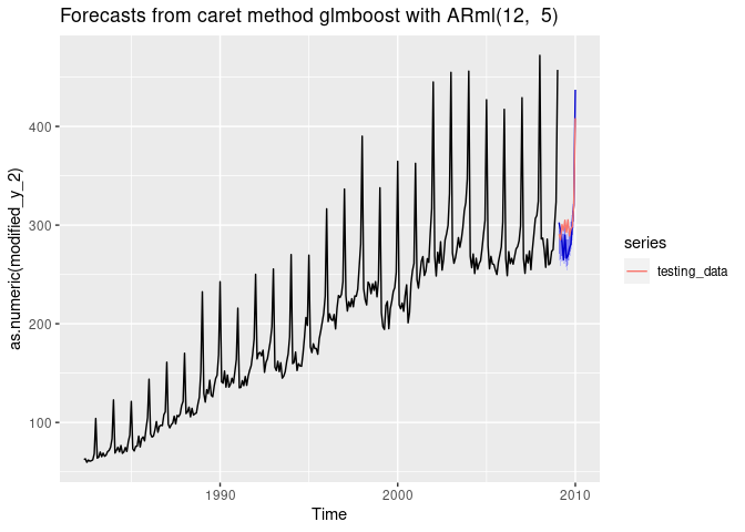
# Forecasting with glmboost
data(retail_wide, package = "caretForecast")
i <- 8
dtlist <- caretForecast::split_ts(retail_wide[,i], test_size = 12)
training_data <- dtlist$train
testing_data <- dtlist$test
fit <- ARml(training_data, max_lag = 12, caret_method = "glmboost",
verbose = FALSE)
#> Loading required package: lattice
#> Loading required package: ggplot2
forecast(fit, h = length(testing_data), level = c(80,95), PI = TRUE)-> fc
accuracy(fc, testing_data)
#> ME RMSE MAE MPE MAPE MASE
#> Training set 0.8868074 16.39661 11.65025 -0.3620986 5.702257 0.7559694
#> Test set 8.3976171 20.15546 17.20306 3.0153042 5.572722 1.1162843
#> ACF1 Theil's U
#> Training set 0.5707204 NA
#> Test set 0.3971016 0.7547318
autoplot(fc) +
autolayer(testing_data, series = "testing_data")
## NOTE : Promotions, holidays, and other external variables can be added in the model via xreg argument. Please look at the documentation of ARml.

# Forecasting with cubist regression

i <- 9

data(retail_wide, package = "caretForecast")

dtlist <- caretForecast::split_ts(retail_wide[,i], test_size = 12)

training_data <- dtlist$train

testing_data <- dtlist$test

fit <- ARml(training_data, max_lag = 12, caret_method = "cubist",
            verbose = FALSE)

forecast(fit, h = length(testing_data), level = c(80,95), PI = TRUE)-> fc

accuracy(fc, testing_data)
#>                     ME     RMSE      MAE         MPE     MAPE      MASE
#> Training set 0.3452345 16.39877 12.22406 -0.08475644 2.533889 0.4073634
#> Test set     2.5562312 14.21461 12.39887  0.24907619 1.592606 0.4131888
#>                    ACF1 Theil's U
#> Training set  0.2309758        NA
#> Test set     -0.1450719 0.1701567
autoplot(fc) +
  autolayer(testing_data, series = "testing_data")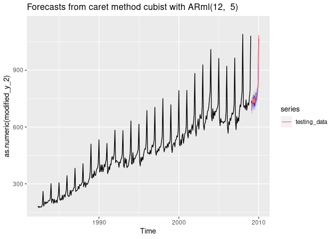
# Forecasting using Support Vector Machines with Linear Kernel

data(retail_wide, package = "caretForecast")

i <- 9

dtlist <- caretForecast::split_ts(retail_wide[,i], test_size = 12)

training_data <- dtlist$train

testing_data <- dtlist$test

fit <- ARml(training_data, max_lag = 12, caret_method = "svmLinear2",
            verbose = FALSE, pre_process = c("scale", "center"))

forecast(fit, h = length(testing_data), level = c(80,95), PI = TRUE)-> fc

accuracy(fc, testing_data)
#>                     ME     RMSE      MAE        MPE     MAPE      MASE
#> Training set  1.086666 15.67422 11.87520 0.06663619 2.497392 0.3957375
#> Test set     10.671509 16.75893 12.72986 1.33830385 1.611293 0.4242188
#>                     ACF1 Theil's U
#> Training set  0.09739853        NA
#> Test set     -0.27328009 0.2062128
autoplot(fc) +
  autolayer(testing_data, series = "testing_data")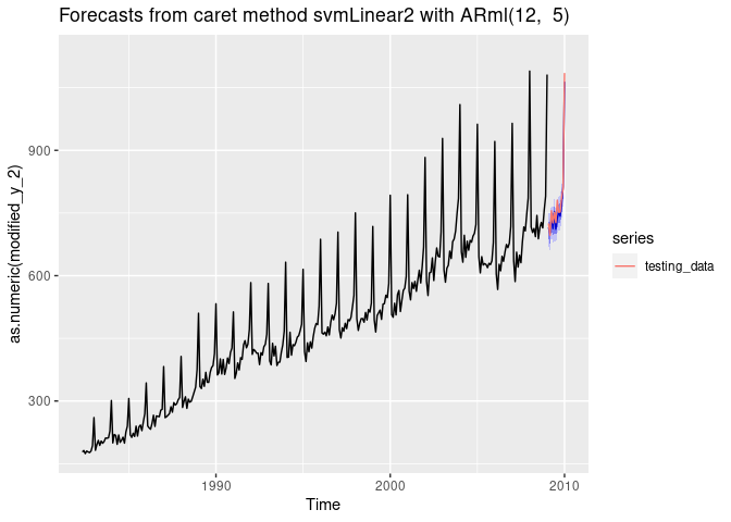
get_var_imp(fc)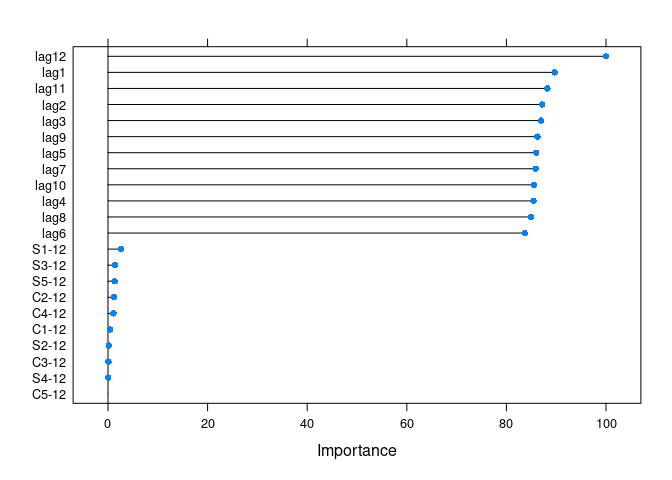
get_var_imp(fc, plot = F)
#> loess r-squared variable importance
#>
#>   only 20 most important variables shown (out of 22)
#>
#>         Overall
#> lag12 100.00000
#> lag1   89.70809
#> lag11  88.21434
#> lag2   87.15896
#> lag3   86.95035
#> lag9   86.22539
#> lag5   85.98743
#> lag7   85.86392
#> lag10  85.56408
#> lag4   85.44561
#> lag8   84.95210
#> lag6   83.66422
#> S1-12   2.62893
#> S3-12   1.38199
#> S5-12   1.32829
#> C2-12   1.21307
#> C4-12   1.09981
#> C1-12   0.44682
#> S2-12   0.14723
#> C3-12   0.09562
# Forecasting using Ridge Regression
data(retail_wide, package = "caretForecast")

i <- 8

dtlist <- caretForecast::split_ts(retail_wide[,i], test_size = 12)

training_data <- dtlist$train

testing_data <- dtlist$test

fit <- ARml(training_data, max_lag = 12, caret_method = "ridge",
            verbose = FALSE)

forecast(fit, h = length(testing_data), level = c(80,95), PI = TRUE)-> fc

accuracy(fc, testing_data)
#>                     ME     RMSE      MAE        MPE     MAPE      MASE
#> Training set 0.1414756  8.88367  6.44208 -0.0953757 3.126316 0.4180182
#> Test set     0.9965672 17.71459 13.30744  0.7019753 4.092068 0.8635023
#>                     ACF1 Theil's U
#> Training set 0.004518837        NA
#> Test set     0.389409945 0.6513039
autoplot(fc) +
  autolayer(testing_data, series = "testing_data")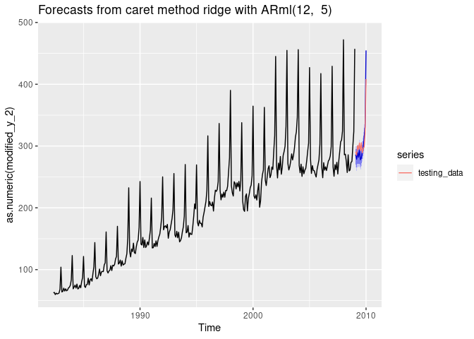
get_var_imp(fc)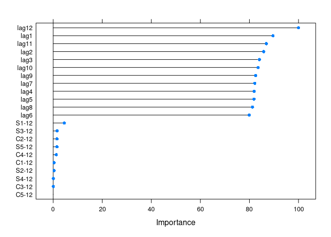
get_var_imp(fc, plot = F)
#> loess r-squared variable importance
#>
#>   only 20 most important variables shown (out of 22)
#>
#>         Overall
#> lag12 100.00000
#> lag1   89.57697
#> lag11  86.89260
#> lag2   85.81967
#> lag3   84.07269
#> lag10  83.53358
#> lag9   82.52774
#> lag7   82.18917
#> lag4   81.93730
#> lag5   81.85290
#> lag8   81.22696
#> lag6   79.96364
#> S1-12   4.51371
#> S3-12   1.59063
#> C2-12   1.54661
#> S5-12   1.53004
#> C4-12   1.24044
#> C1-12   0.38784
#> S2-12   0.35446
#> S4-12   0.07244