README

The envi package is a suite of R functions to estimate the ecological niche of a species and predict the spatial distribution of the ecological niche – a version of environmental interpolation – with spatial kernel density estimation techniques. A two group comparison (e.g., presence and absence locations of a single species) is conducted using the spatial relative risk function that is estimated using the sparr package. Internal cross-validation and basic visualization are also supported.

Installation

Available functions

Function	Description
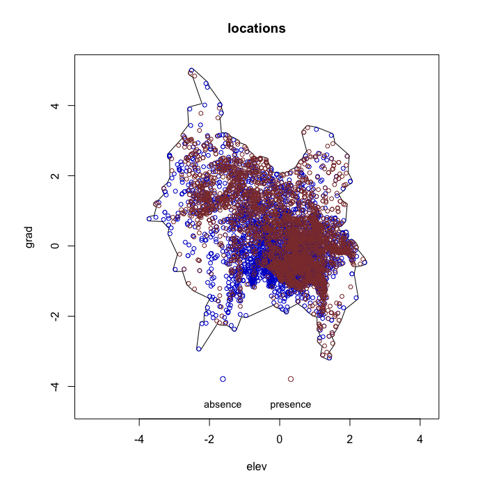
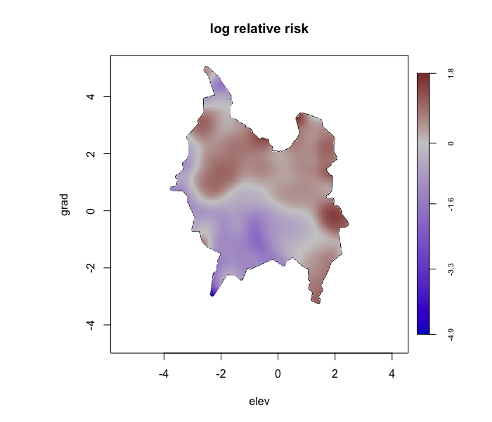
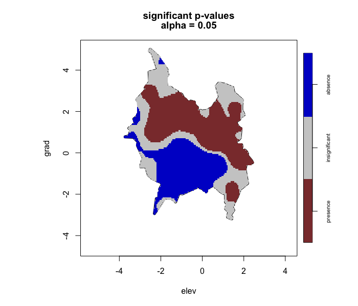
`lrren`	Main function. Estimate an ecological niche using the spatial relative risk function and predict its location in geographic space.
`perlrren`	Sensitivity analysis for `lrren` whereby observation locations are spatially perturbed (“jittered”) with specified radii, iteratively.
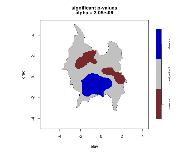
`plot_obs`	Display multiple plots of the estimated ecological niche from `lrren` output.
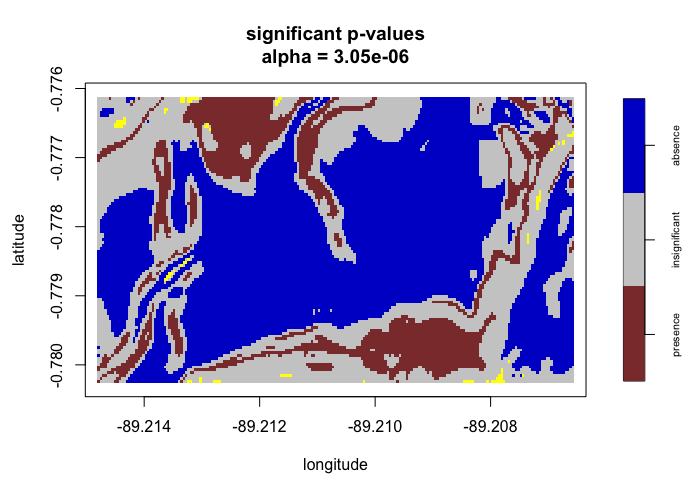
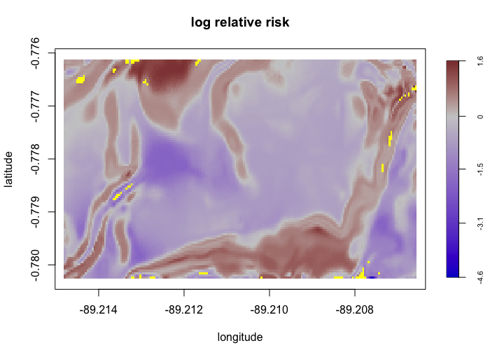
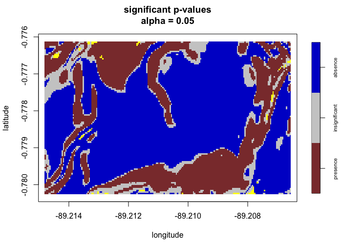
`plot_predict`	Display multiple plots of the predicted spatial distribution from `lrren` output.
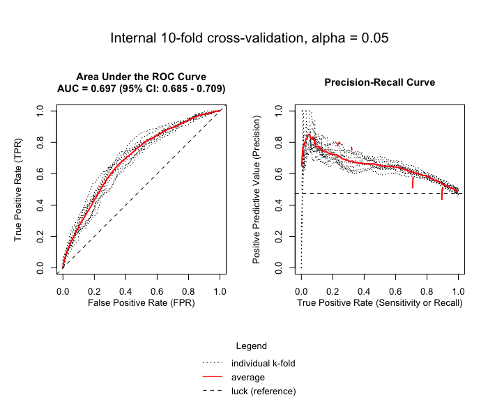
`plot_cv`	Display multiple plots of internal k-fold cross-validation diagnostics from `lrren` output.
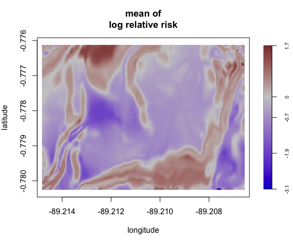
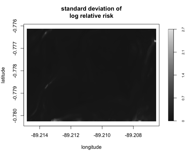
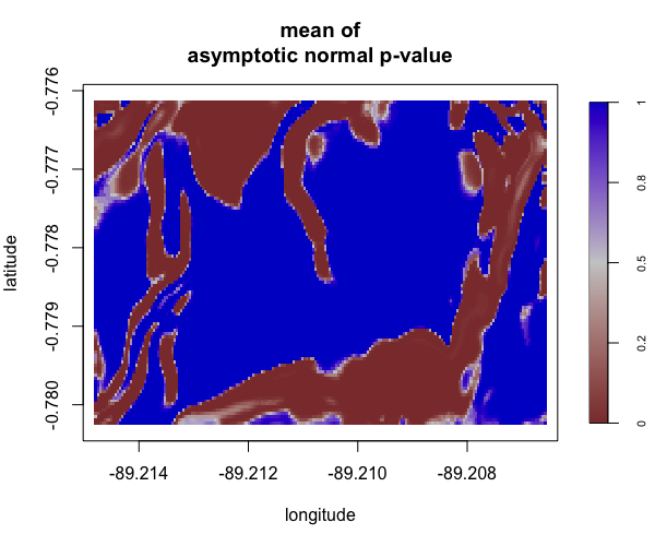
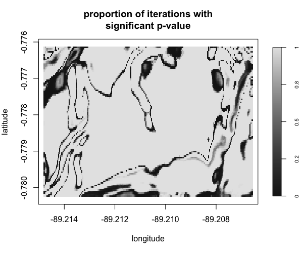
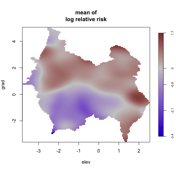
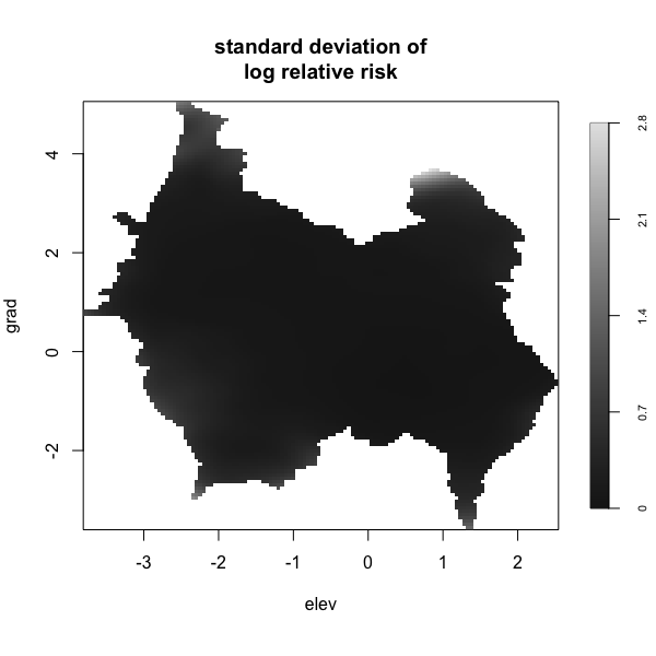
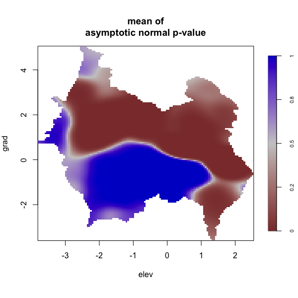
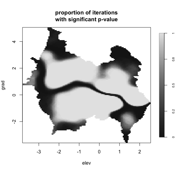
`plot_perturb`	Display multiple plots of output from `perlrren` including prediced spatial distribution of the summary statistics.
`div_plot`	Called within `plot_obs`, `plot_predict`, and `plot_perturb`, provides functionality for basic visualization of surfaces with diverging color palettes.
`seq_plot`	Called within `plot_perturb`, provides functionality for basic visualization of surfaces with sequential color palettes.
`pval_correct`	Called within `lrren` and `perlrren`, calculates various multiple testing corrections for the alpha level.

Authors

Usage

For the lrren() function

set.seed(1234) # for reproducibility

# ------------------ #
# Necessary packages #
# ------------------ #

library(envi)
library(raster)
library(spatstat.data)
library(spatstat.geom)
library(spatstat.random)

# -------------- #
# Prepare inputs #
# -------------- #

# Using the 'bei' and 'bei.extra' data within {spatstat.data}

# Environmental Covariates
elev <- spatstat.data::bei.extra[[1]]
grad <- spatstat.data::bei.extra[[2]]
elev$v <- scale(elev)
grad$v <- scale(grad)
elev_raster <- raster::raster(elev)
grad_raster <- raster::raster(grad)

# Presence data
presence <- spatstat.data::bei
spatstat.geom::marks(presence) <- data.frame("presence" = rep(1, presence$n),
                                        "lon" = presence$x,
                                        "lat" = presence$y)
spatstat.geom::marks(presence)$elev <- elev[presence]
spatstat.geom::marks(presence)$grad <- grad[presence]

# (Pseudo-)Absence data
absence <- spatstat.random::rpoispp(0.008, win = elev)
spatstat.geom::marks(absence) <- data.frame("presence" = rep(0, absence$n),
                                            "lon" = absence$x,
                                            "lat" = absence$y)
spatstat.geom::marks(absence)$elev <- elev[absence]
spatstat.geom::marks(absence)$grad <- grad[absence]

# Combine
obs_locs <- spatstat.geom::superimpose(presence, absence, check = FALSE)
obs_locs <- spatstat.geom::marks(obs_locs)
obs_locs$id <- seq(1, nrow(obs_locs), 1)
obs_locs <- obs_locs[ , c(6, 2, 3, 1, 4, 5)]

# Prediction Data
predict_locs <- data.frame(raster::rasterToPoints(elev_raster))
predict_locs$layer2 <- raster::extract(grad_raster, predict_locs[, 1:2])

# ----------- #
# Run lrren() #
# ----------- #

test1 <- envi::lrren(obs_locs = obs_locs,
                     predict_locs = predict_locs,
                     predict = TRUE,
                     verbose = TRUE,
                     cv = TRUE)
              
# -------------- #
# Run plot_obs() #
# -------------- #

envi::plot_obs(test1)

# ------------------ #
# Run plot_predict() #
# ------------------ #

envi::plot_predict(test1,
                   cref0 = "EPSG:5472",
                   cref1 = "EPSG:4326")

# ------------- #
# Run plot_cv() #
# ------------- #

envi::plot_cv(test1)

# -------------------------------------- #
# Run lrren() with Bonferroni correction #
# -------------------------------------- #

test2 <- envi::lrren(obs_locs = obs_locs,
                     predict_locs = predict_locs,
                     predict = TRUE,
                     p_correct = "Bonferroni")

# Note: Only showing third plot
envi::plot_obs(test2)

# Note: Only showing second plot
envi::plot_predict(test2,
                   cref0 = "EPSG:5472",
                   cref1 = "EPSG:4326")

# Note: plot_cv() will display the same results because cross-validation only performed for the log relative risk estimate

For the perlrren() function

set.seed(1234) # for reproducibility

# ------------------ #
# Necessary packages #
# ------------------ #

library(envi)
library(raster)
library(spatstat.data)
library(spatstat.geom)
library(spatstat.random)

# -------------- #
# Prepare inputs #
# -------------- #

# Using the 'bei' and 'bei.extra' data within {spatstat.data}

# Scale environmental covariates
ims <- spatstat.data::bei.extra
ims[[1]]$v <- scale(ims[[1]]$v)
ims[[2]]$v <- scale(ims[[2]]$v)

# Presence data
presence <- spatstat.data::bei
spatstat.geom::marks(presence) <- data.frame("presence" = rep(1, presence$n),
                                             "lon" = presence$x,
                                             "lat" = presence$y)

# (Pseudo-)Absence data
absence <- spatstat.random::rpoispp(0.008, win = ims[[1]])
spatstat.geom::marks(absence) <- data.frame("presence" = rep(0, absence$n),
                                            "lon" = absence$x,
                                            "lat" = absence$y)

# Combine and create 'id' and 'levels' features
obs_locs <- spatstat.geom::superimpose(presence, absence, check = FALSE)
spatstat.geom::marks(obs_locs)$id <- seq(1, obs_locs$n, 1)
spatstat.geom::marks(obs_locs)$levels <- as.factor(stats::rpois(obs_locs$n, lambda = 0.05))
spatstat.geom::marks(obs_locs) <- spatstat.geom::marks(obs_locs)[ , c(4, 2, 3, 1, 5)]

# -------------- #
# Run perlrren() #
# -------------- #

# Uncertainty in observation locations
## Most observations within 10 meters
## Some observations within 100 meters
## Few observations within 500 meters

test3 <- envi::perlrren(obs_ppp = obs_locs,
                        covariates = ims,
                        radii = c(10,100,500),
                        verbose = FALSE, # may not be availabe if parallel = TRUE
                        parallel = TRUE,
                        n_sim = 100)
                 
# ------------------ #
# Run plot_perturb() #
# ------------------ #

envi::plot_perturb(test3,
                   cref0 = "EPSG:5472",
                   cref1 = "EPSG:4326",
                   cov_labs = c("elev", "grad"))