![]()
![]()
With {fHMM} you can detect and characterize financial market regimes in financial time series by applying hidden Markov Models (HMMs). The functionality and the model is documented in detail here. Below, you can find a first application to the German stock index DAX.
You can install the released version of {fHMM} from CRAN with:
install.packages("fHMM")And the development version from GitHub with:
# install.packages("devtools")
devtools::install_github("loelschlaeger/fHMM")We welcome contributions! Please submit bug reports and feature requests as issues and extensions as pull request from a branch forked from main.
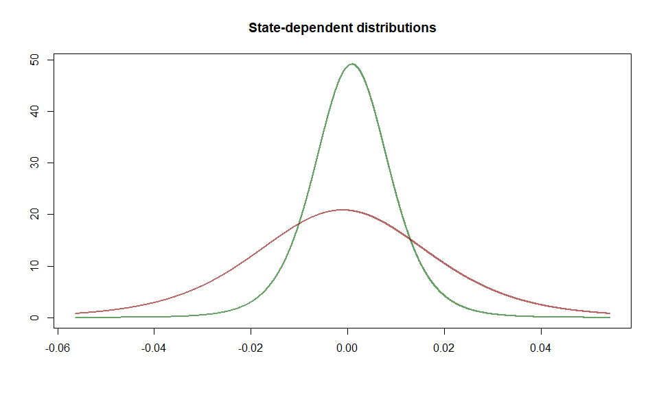
We fit a 2-state HMM with state-dependent t-distributions to the DAX log-returns from 2000 to 2020. The states can be interpreted as proxies for bearish and bullish markets.
The package has a build-in function to download the data from Yahoo Finance:
path <- paste0(tempdir(),"/dax.csv")
download_data(symbol = "^GDAXI", file = path, verbose = FALSE)
We first need to define the model by setting some
controls:
controls <- list(
  states = 2,
  sdds   = "t",
  data   = list(file        = path,
                date_column = "Date",
                data_column = "Close",
                logreturns  = TRUE,
                from        = "2000-01-01",
                to          = "2020-12-31")
)
controls <- set_controls(controls)
The function prepare_data() prepares the data for
estimation:
data <- prepare_data(controls)
summary(data)
#> Summary of fHMM empirical data
#> * number of observations: 5371
#> * data source: dax.csv
#> * date column: Date
#> * log returns: TRUE
We fit the model and subsequently decode the hidden states:
model <- fit_model(data, ncluster = 7)
#> Checking start values
#> Maximizing likelihood
#> Computing Hessian
#> Fitting completed
model <- decode_states(model)
#> Decoded states
summary(model)
#> Summary of fHMM model
#>
#> simulated hierarchy LL AIC BIC
#> 1 FALSE FALSE 15920.25 -31824.5 -31771.79
#>
#> State-dependent distributions:
#> t()
#>
#> Estimates:
#> lb estimate ub
#> Gamma_2.1 0.0113550 0.0179502 2.827e-02
#> Gamma_1.2 0.0056213 0.0089654 1.427e-02
#> mu_1 0.0005939 0.0009008 1.208e-03
#> mu_2 -0.0020763 -0.0010611 -4.585e-05
#> sigma_1 0.0073792 0.0078062 8.258e-03
#> sigma_2 0.0170391 0.0184230 1.992e-02
#> df_1 5.0194906 6.4223618 8.217e+00
#> df_2 4.9532404 6.6609735 8.957e+00
#>
#> States:
#> decoded
#> 1 2
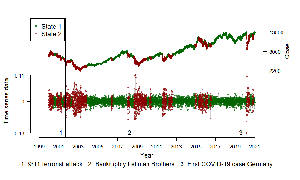
#> 3645 1726Having estimated the model, we can visualize the state-dependent distributions and the decoded time series:
events <- fHMM_events(
  list(dates = c("2001-09-11", "2008-09-15", "2020-01-27"),
       labels = c("9/11 terrorist attack", "Bankruptcy Lehman Brothers", "First COVID-19 case Germany"))
)
plot(model, plot_type = c("sdds","ts"), events = events)