The goal of fcirt is to estimate forced choice models using Bayesian method. Specifically, the Multi-Unidimensional Pairwise Preference (MUPP) model is estimated using the R package rstan that utilizes the Hamiltonian Monte Carlo sampling algorithm. Four functions (i.e., fcirt( ), extract( ), information( ), and bayesplot( )) are provided for model estimation, results extraction, item and test information computation, and Bayesian diagnostic plottings, respectively.
You can install the development version of fcirt from GitHub:
This is a basic example which shows you how to prepare data, fit the model, extract and plot results:
library(fcirt)

## basic example code
## Step 1: Input data
# 1.1 Response data in wide format
fcirt.Data <- c(1,0,0,1,1,1,1,1,1,1,0,1,1,0,1,1,0,0,0,0,0,0,1,1,1,0,1,1,1,1,0,1,1,1,0,1,1,0,1,1)
fcirt.Data <- matrix(fcirt.Data,nrow = 10)
fcirt.Data
#>       [,1] [,2] [,3] [,4]
#>  [1,]    1    0    0    0
#>  [2,]    0    1    0    1
#>  [3,]    0    1    1    1
#>  [4,]    1    0    1    1
#>  [5,]    1    1    1    0
#>  [6,]    1    1    0    1
#>  [7,]    1    0    1    1
#>  [8,]    1    0    1    0
#>  [9,]    1    0    1    1
#> [10,]    1    0    1    1

# 1.2 A two-column data matrix: the first column is the statement number for statement s; the second column is the statement number for statement t.
pairmap <- c(1,3,5,7,2,4,6,8)
pairmap <- matrix(pairmap,ncol = 2)
pairmap
#>      [,1] [,2]
#> [1,]    1    2
#> [2,]    3    4
#> [3,]    5    6
#> [4,]    7    8

# 1.3 A column vector mapping each statement to each trait.
ind <- c(1,2,1,2,1,2,2,1)

# 1.4 A three-column matrix containing initial values for the three statement parameters (alpha, delta, tau) respectively. If using the direct MUPP estimation approach, 1 and -1 for alphas and taus are recommended and -1 or 1 for deltas are recommended depending on the signs of the statements. If using the two-step estimation approach, pre-estimated statement parameters are used as the initial values. The R package **bmggum** (Tu et al., 2021) can be used to estimate statement parameters for the two-step approach.
ParInits <- c(1, 1, 1, 1, 1, 1, 1, 1, 1, -1, 1, 1, 1, -1, 1, 1, -1, -1, -1, -1, -1, -1, -1, -1)
ParInits <- matrix(ParInits, ncol = 3)
ParInits
#>      [,1] [,2] [,3]
#> [1,]    1    1   -1
#> [2,]    1   -1   -1
#> [3,]    1    1   -1
#> [4,]    1    1   -1
#> [5,]    1    1   -1
#> [6,]    1   -1   -1
#> [7,]    1    1   -1
#> [8,]    1    1   -1

## Step 2: Fit the MUPP model
mod <- fcirt(fcirt.Data=fcirt.Data, pairmap=pairmap, ind=ind, ParInits=ParInits, iter=1000)

## Step 3: Extract the estimated results
# 3.1 Extract the theta estimates
theta <- extract(x=mod, pars='theta')
# Turn the theta estimates into p*trait matrix where p equals sample size and trait equals the number of latent traits
theta <- theta[,1]
# nrow=trait
theta <- matrix(theta, nrow=2)
theta <- t(theta)
# theta estimates in p*trait matrix format
theta
#>               [,1]        [,2]
#>  [1,] -0.023326651 -0.03055898
#>  [2,]  0.023196544  0.02679090
#>  [3,] -0.014954009  0.03139395
#>  [4,] -0.017056012 -0.01386742
#>  [5,] -0.008155243 -0.03766694
#>  [6,]  0.058712369 -0.01697841
#>  [7,] -0.022276577  0.00689250
#>  [8,]  0.036137392  0.03138213
#>  [9,]  0.006967824 -0.01321674
#> [10,] -0.023923473  0.01056224
# 3.2 Extract the tau estimates
tau <- extract(x=mod, pars='tau')
tau <- tau[,1]
tau
#>     tau[1]     tau[2]     tau[3]     tau[4]     tau[5]     tau[6]     tau[7]
#> -2.0767845 -0.9670536 -1.2123404 -1.5029586 -1.7202191 -1.0379493 -1.7797779
#>     tau[8]
#> -1.0244982

## Step 4: Plottings
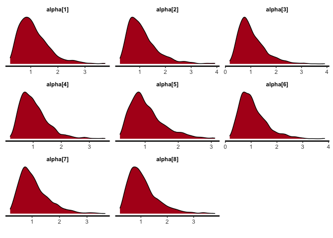
# 4.1 Obtain the density plots for alpha
bayesplot(x=mod, pars='alpha', plot='density', inc_warmup=FALSE)
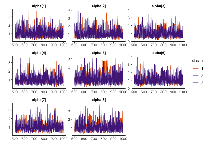
# 4.2 Obtain the trace plots for alpha
bayesplot(x=mod, pars='alpha', plot='trace', inc_warmup=FALSE)
## Step 5: Item information
# 5.1 Obtain item information for item 1-3
OII <- information(x=mod, approach="direct", information="item", items=1:3)
OII
#> [1] 0.3935772 0.4049316 0.4042282
# 5.2 Obtain test information
OTI <- information(x=mod, approach="direct", information="test")
OTI
#> [1] 1.608332