The goal of forrel is to provide forensic pedigree computations and relatedness inference from genetic marker data. The forrel package is part of the ped suite, a collection of R packages for pedigree analysis.
The most important analyses currently supported by forrel are:
missingPersonPlot()missingPersonEP()missingPersonIP()MPPsims()powerPlot()Familias software.To get the current official version of forrel, install from CRAN as follows:
Alternatively, you can obtain the latest development version from GitHub:
# install.packages("devtools") # install devtools if needed
devtools::install_github("magnusdv/forrel")In this short introduction, we first demonstrate simulation of marker data for a pair of siblings. Then - pretending the relationship is unknown to us - we estimate the relatedness between the brothers using the simulated data. If all goes well, the estimate should be close to the expected value for siblings.
Create the pedigree
We start by creating and plotting a pedigree with two brothers, named bro1 and bro2.

Marker simulation
Now let us simulate the genotypes of 100 independent SNPs for the brothers. Each SNP has alleles 1 and 2, with equal frequencies by default. This is an example of unconditional simulation, since we don’t give any genotypes to condition on. Unconditional simulation is performed by simple gene dropping, i.e., by drawing random alleles independently for the parents, followed by a “Mendelian coin toss” in each parent-child transmission.
x = markerSim(x, N = 100, ids = bros, alleles = 1:2, seed = 1234)
#> Unconditional simulation of 100 autosomal markers.
#> Individuals: bro1, bro2
#> Allele frequencies:
#>    1   2
#>  0.5 0.5
#> Mutation model: No
#>
#> Simulation finished.
#> Calls to `likelihood()`: 0.
#> Total time used: 0.13 seconds.
Note 1: The seed argument is passed onto the random number generator. If you use the same seed, you should get exactly the same results.
Note 2: To suppress the informative messages printed during simulation, add verbose = FALSE to the function call.
The pedigree x now has 100 markers attached to it. The genotypes of the first few markers are shown when printing x to the screen:
x
#>    id fid mid sex <1> <2> <3> <4> <5>
#>     1   *   *   1 -/- -/- -/- -/- -/-
#>     2   *   *   2 -/- -/- -/- -/- -/-
#>  bro1   1   2   1 1/1 1/2 1/1 1/2 2/2
#>  bro2   1   2   1 1/1 1/2 1/1 1/2 2/2
#> Only 5 (out of 100) markers are shown.
Estimation of IBD coefficients
The ibdEstimate() function estimates the coefficients of identity-by-descent (IBD) between pairs of individuals, from the available marker data.
k = ibdEstimate(x, ids = bros)
#> Estimating 'kappa' coefficients
#> Initial search value: (0.333, 0.333, 0.333)
#> Pairs of individuals: 1
#> bro1 vs. bro2: estimate = (0.149, 0.551, 0.3), iterations = 16
#> Total time: 0.0146 secs
k
#> id1 id2 N k0 k1 k2
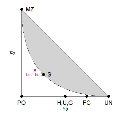
#> 1 bro1 bro2 100 0.1486 0.55139 0.30002The theoretical expectation for non-inbred full siblings is (κ0,κ1,κ2) = (0.25,0.5,0.25). To get a visual sense of how close our estimate is, it is instructive to plot it in the IBD triangle: