![]()
The geostan R package supports a complete spatial analysis workflow with Bayesian models for areal data, including a suite of functions for visualizing spatial data and model results. For demonstrations and discussion, see the package help pages and vignettes on spatial autocorrelation and spatial measurement error models.
The package is designed primarily to support public health research with spatial data; see the surveil R package for time series analysis of public health surveillance data.
geostan is an interface to Stan, a state-of-the-art platform for Bayesian inference.
Model small-area incidence rates with mortality or disease data recorded across areal units like states, counties, or census tracts.
Incorporate information on data reliability, such as standard errors of American Community Survey estimates, into any geostan model.
Vital statistics and disease surveillance systems like CDC Wonder censor case counts that fall below a threshold number; geostan can model disease or mortality risk with censored observations.
Tools for visualizing and measuring spatial autocorrelation and map patterns, for exploratory analysis and model diagnostics. Visual diagnostics also support the evaluation of survey data quality and observational error models.
Compatible with a suite of high-quality R packages for Bayesian inference and model evaluation.
Tools for building custom spatial models in Stan.
Install geostan from CRAN using:
install.packages("geostan")Linux users may also install from source:
remotes::install_github("connordonegan/geostan")Then run:
rstantools::rstan_config()Load the package and the georgia county mortality data
set (ages 55-64, years 2014-2018):
library(geostan)
#> This is geostan version 0.2.1
#>
#> Attaching package: 'geostan'
#> The following object is masked from 'package:base':
#>
#>     gamma
data(georgia)
The sp_diag function provides visual summaries of
spatial data, including a histogram, Moran scatter plot, and map:
sp_diag(georgia$rate.female, georgia)
#> 3 NA values found in x. They will be dropped from the data before creating the Moran plot. If matrix w was row-standardized, it no longer is. To address this, you can use a binary connectivity matrix, using style = 'B' in shape2mat.
#> Warning: Removed 3 rows containing non-finite values (stat_bin).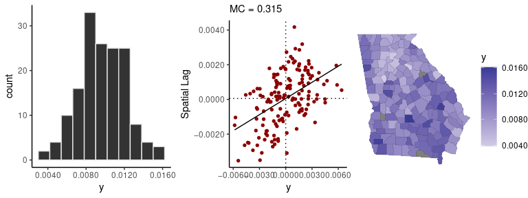
There are three censored observations in the georgia
female mortality data, which means there were 9 or fewer deaths in those
counties. The following code fits a spatial conditional autoregressive
(CAR) model to female county mortality data. By using the
censor_point argument we include our information on the
censored observations to obtain results for all counties:
A <- shape2mat(georgia, style = "B")
cars <- prep_car_data(A)
#> Range of permissible rho values:  -1.661134 1
fit <- stan_car(deaths.female ~ offset(log(pop.at.risk.female)),
                censor_point = 9,
        data = georgia,
        car_parts = cars,
        family = poisson(),
        cores = 4, # for multi-core processing
        refresh = 0) # to silence some printing
#>
#> *Setting prior parameters for intercept
#> Distribution: normal
#>   location scale
#> 1     -4.7     5
#>
#> *Setting prior for CAR scale parameter (car_scale)
#> Distribution: student_t
#>   df location scale
#> 1 10        0     3
#>
#> *Setting prior for CAR spatial autocorrelation parameter (rho)
#> Distribution: uniform
#>   lower upper
#> 1  -1.7     1
Passing a fitted model to the sp_diag function will
return a set of diagnostics for spatial models:
sp_diag(fit, georgia, w = A)
#> 3 NA values found in x. They will be dropped from the data before creating the Moran plot. If matrix w was row-standardized, it no longer is. To address this, you can use a binary connectivity matrix, using style = 'B' in shape2mat.
#> Warning: Removed 3 rows containing missing values (geom_pointrange).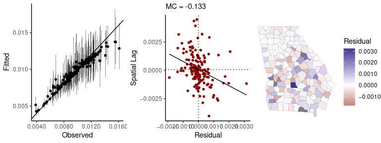
The print method returns a summary of the probability
distributions for model parameters, as well as Markov chain Monte Carlo
(MCMC) diagnostics from Stan (Monte Carlo standard errors of the mean
se_mean, effective sample size n_eff, and the
R-hat statistic Rhat):
print(fit)
#> Spatial Model Results
#> Formula: deaths.female ~ offset(log(pop.at.risk.female))
#> Spatial method (outcome):  CAR
#> Likelihood function:  poisson
#> Link function:  log
#> Residual Moran Coefficient:  0.000228
#> WAIC:  1292.1
#> Observations:  159
#> Data models (ME): none
#> Inference for Stan model: foundation.
#> 4 chains, each with iter=2000; warmup=1000; thin=1;
#> post-warmup draws per chain=1000, total post-warmup draws=4000.
#>
#>             mean se_mean    sd   2.5%    25%    50%    75%  97.5% n_eff  Rhat
#> intercept -4.674   0.002 0.089 -4.846 -4.718 -4.674 -4.631 -4.496  1648 1.002
#> car_rho    0.923   0.001 0.058  0.778  0.895  0.935  0.966  0.995  3618 1.000
#> car_scale  0.457   0.001 0.035  0.393  0.432  0.455  0.480  0.531  3855 1.000
#>
#> Samples were drawn using NUTS(diag_e) at Thu Jun 30 12:41:42 2022.
#> For each parameter, n_eff is a crude measure of effective sample size,
#> and Rhat is the potential scale reduction factor on split chains (at
#> convergence, Rhat=1).
More demonstrations can be found in the package help pages and vignettes.