ggblanket

Overview

{ggblanket} is a package of {ggplot2} wrapper functions to simplify visualisation.

To do this, the {ggblanket} package:

uses gg_* functions that wrap a single ggplot2::geom_* function
merges col and fill aesthetics into a single col argument
customises colours via pal and alpha arguments consistently
provides a facet argument to facet by a single variable
provides an additional facet2 argument to facet in a grid
provides prefixed arguments to help find arguments
uses nice numeric/date default scales.
provides a theme argument for customisation.
provides a gg_theme function to create a quick theme.
arranges horizontal plot labels to be in correct order
converts unspecified titles to snakecase::to_sentence
provides a gg_blank function for extra flexibility
supports nice plotly::ggplotly tooltips
provides access to all other geom_* arguments via ...
is useful for creating customised functions with your own defaults

If you would like to show your appreciation for {ggblanket}, you can give this repository a star, or even buy me a coffee.

Website

Click here for the {ggblanket} website.

Installation

Install either from CRAN with:

install.packages("ggblanket")

Or install the development version with:

# install.packages("devtools")
devtools::install_github("davidhodge931/ggblanket")

Examples

library(dplyr)
library(ggplot2)
library(ggblanket)
library(palmerpenguins)

{ggblanket} uses gg_* functions that wrap a single ggplot2::geom_* function.

iris %>%
  mutate(Species = stringr::str_to_sentence(Species)) %>% 
  gg_point(
    x = Sepal.Width, 
    y = Sepal.Length, 
    col = Species)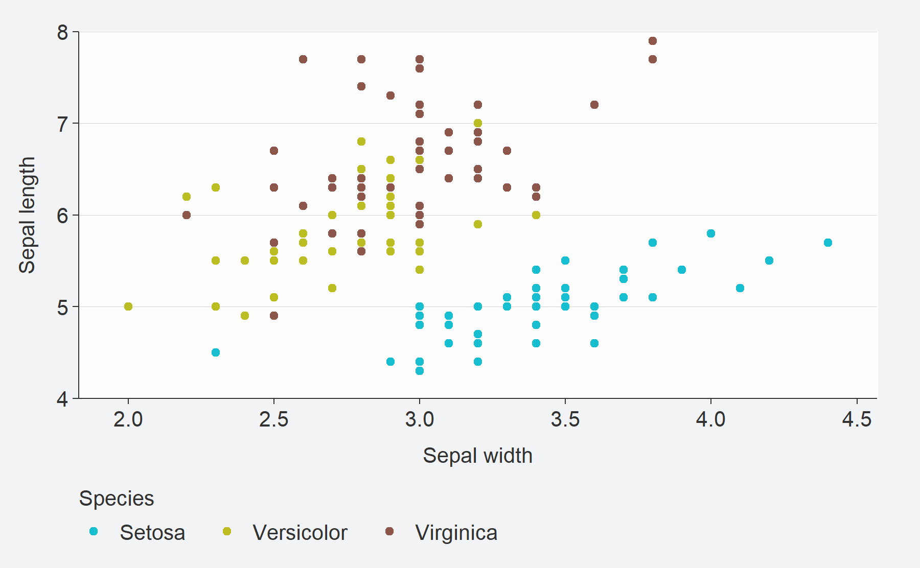

{ggblanket} merges col and fill aesthetics into a single col argument.

penguins %>% 
  gg_histogram(
    x = body_mass_g, 
    col = species)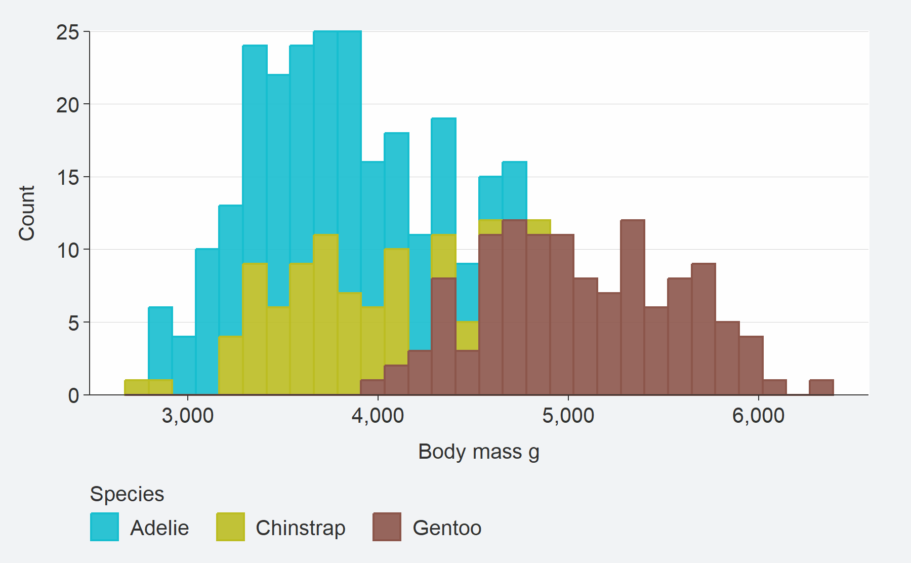

{ggblanket} customises colours via pal and alpha arguments consistently.

These arguments are the same regardless of whether a col variable is specified. If more colours are provided than needed by the pal argument, then the excess colours will just be dropped. Note all colours specified by the pal argument will inherit to any further ggplot2::geom_* layers added.

penguins %>% 
  mutate(sex = stringr::str_to_sentence(sex)) %>% 
  group_by(species, sex) %>% 
  summarise(body_mass_g = mean(body_mass_g, na.rm = TRUE)) %>% 
  gg_col(
    x = species, 
    y = body_mass_g, 
    col = sex, 
    position = position_dodge2(preserve = "single"),
    pal = c("#1B9E77", "#9E361B"))

{ggblanket} provides a facet argument to facet by a single variable.

penguins %>% 
  tidyr::drop_na(sex) %>%
  mutate(sex = stringr::str_to_sentence(sex)) %>% 
  gg_violin(
    x = sex, 
    y = body_mass_g, 
    facet = species, 
    y_include = 0, 
    y_breaks = scales::breaks_width(1000),
    pal = "#1B9E77")

{ggblanket} provides an additional facet2 argument to facet in a grid.

penguins %>% 
  tidyr::drop_na(sex) %>% 
  mutate(sex = stringr::str_to_sentence(sex)) %>% 
  gg_point(
    x = bill_length_mm, 
    y = body_mass_g,
    col = sex,
    facet = species,
    facet2 = sex, 
    y_breaks = scales::breaks_width(1500), 
    size = 1)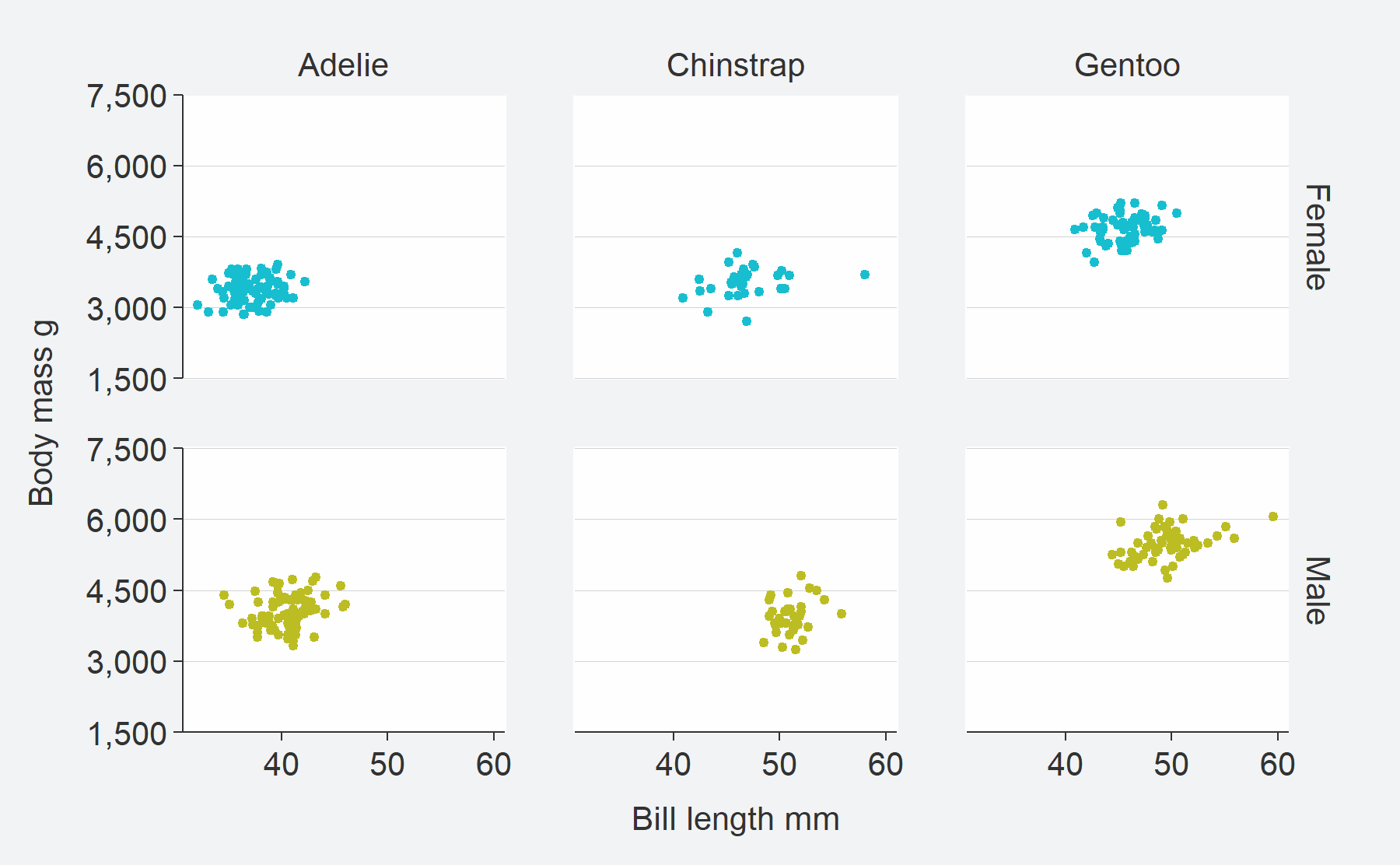

{ggblanket} provides prefixed arguments to help find arguments.

This is designed to work with the Rstudio autocomplete to help you find the adjustment you need. Press the tab key after typing x_,y_, col_ or facet_ to access this. Then use arrow keys, and press tab again to select.

Available arguments are:

*_breaks: Adjust the breaks of an axis
*_expand: Adjust the padding beyond the limits
*_include: Include a value within a scale
*_labels: Adjust the labels on the breaks
*_limits: Adjust the limits
*_trans: Transform an axis
*_sec_axis: Add a secondary axis
col_intervals: Determine intervals to colour by.

penguins %>%
  gg_jitter(
    x = species,
    y = body_mass_g,
    col = flipper_length_mm,
    position = ggplot2::position_jitter(width = 0.2, height = 0, seed = 123), 
    col_intervals = ~ santoku::chop_quantiles(.x, probs = seq(0, 1, 0.25)),
    col_legend_place = "r",
    y_include = 0,
    y_breaks = scales::breaks_width(1500), 
    y_labels = scales::label_number()
  )

{ggblanket} uses nice numeric/date default scales.

Where x variable is categorical and y numeric, the numeric y scale defaults to the limits being the min and max of the breaks, with expand of c(0, 0). Equivalent happens for the horizontal vice versa situation.

Where both x and y are numeric/date, the y scale defaults to the limits being the min and max of the breaks with expand of c(0, 0) - and x scales default to the min and max of the variable with expand of c(0.025, 0.025).

storms %>%
  group_by(year) %>%
  filter(between(year, 1980, 2020)) %>%
  summarise(wind = mean(wind, na.rm = TRUE)) %>%
  gg_line(
    x = year,
    y = wind,
    x_labels = ~.x,
    y_include = 0,
    title = "Storm wind speed",
    subtitle = "USA average storm wind speed, 1980\u20132020",
    y_title = "Wind speed (knots)",
    caption = "Source: NOAA"
  ) +
  geom_point()

{ggblanket} provides a theme argument for customisation.

This allows you to utilise the simplicity of {ggblanket}, while making content that has your required look and feel.

Your theme will control all theme aspects, other than the legend position and direction. You must instead control these within the gg_* function with the col_legend_place argument (e.g. `col_legend_place = "r").

penguins %>%
  mutate(sex = stringr::str_to_sentence(sex)) %>% 
  gg_point(x = bill_depth_mm,
           y = bill_length_mm,
           col = sex,
           facet = species, 
           pal = c("#1B9E77", "#9E361B"), 
           theme = theme_grey())

{ggblanket} provides a gg_theme function to create a quick theme.

The gg_theme function allows you to create a theme that looks similar to the {ggblanket} look and feel.

This includes the following arguments for adjusting gridlines, background colours, text and axis lines and ticks.

storms %>%
  group_by(year) %>%
  filter(between(year, 1980, 2020)) %>%
  summarise(wind = mean(wind, na.rm = TRUE)) %>%
  gg_col(
    x = year,
    y = wind,
    x_labels = ~.x,
    x_expand = c(0, 0),
    theme = gg_theme(
      bg_plot_pal = "white",
      bg_panel_pal = "white",
      grid_h = TRUE))

{ggblanket} arranges horizontal plot labels to be in correct order.

penguins %>%
  tidyr::drop_na(sex) %>% 
  group_by(species, sex, island) %>%
  summarise(body_mass_kg = mean(body_mass_g) / 1000) %>%
  gg_col(
    x = body_mass_kg, 
    y = species, 
    col = sex, 
    facet = island,
    col_labels = snakecase::to_sentence_case, 
    position = "dodge")

{ggblanket} converts unspecified titles to snakecase::to_sentence.

penguins %>%
  group_by(species, sex) %>%
  summarise(across(body_mass_g, ~ round(mean(.x, na.rm = TRUE)), 0)) %>% 
  gg_tile(
    x = sex, 
    y = species, 
    col = body_mass_g, 
    x_labels = snakecase::to_sentence_case,
    pal = pals::brewer.blues(9), 
    width = 0.9,
    height = 0.9,
    col_legend_place = "r",
    title = "Average penguin body mass",
    subtitle = "Palmer Archipelago, Antarctica",
    theme = gg_theme(grid_h = FALSE,
                     bg_plot_pal = "white",
                     axis_pal = "white", 
                     ticks_pal = "white")) +
  geom_text(aes(label = body_mass_g), col = "#232323", size = 3.5)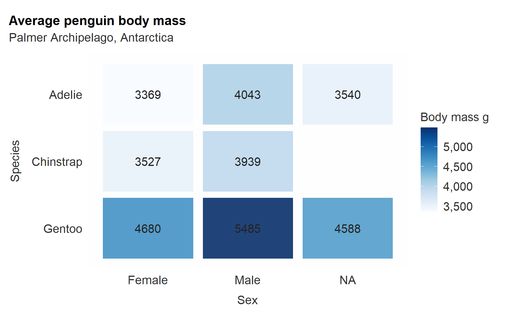

{ggblanket} provides a gg_blank function for extra flexibility.

penguins %>%
  tidyr::drop_na(sex) %>%
  mutate(sex = stringr::str_to_sentence(sex)) %>%
  group_by(species, sex) %>%
  summarise(
    mean = round(mean(bill_length_mm, na.rm = TRUE), 0),
    n = n(),
    se = mean / sqrt(n),
    upper = mean + 1.96 * se,
    lower = mean - 1.96 * se
  ) %>%
  gg_blank(
    x = sex,
    y = mean,
    col = sex,
    facet = species,
    label = mean,
    ymin = lower,
    ymax = upper,
    y_include = 0,
    y_title = "Bill length mm"
  ) +
  geom_col(width = 0.75, alpha = 0.9) +
  geom_errorbar(width = 0.1, colour = pal_na())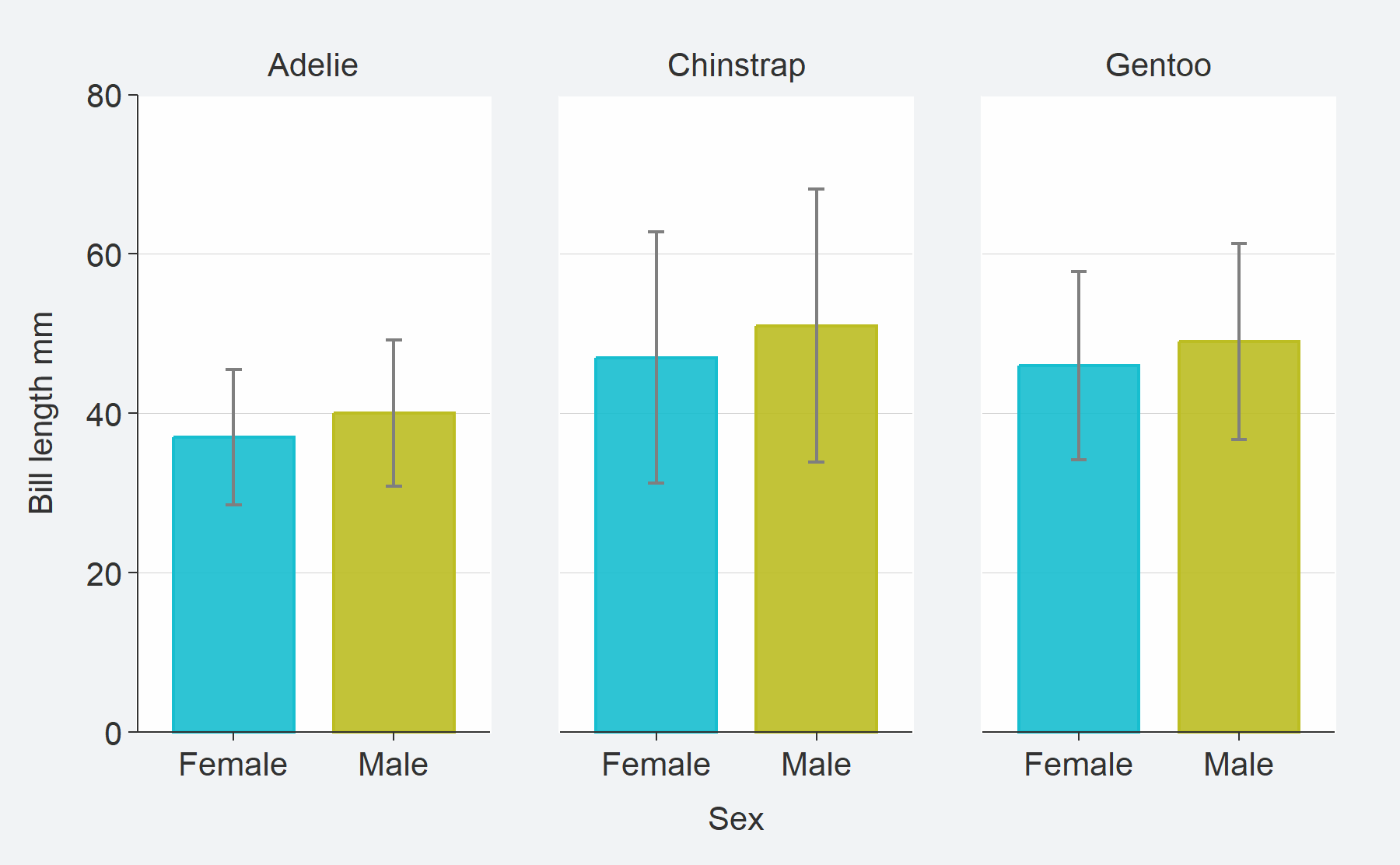

{ggblanket} supports nice plotly::ggplotly tooltips.

The add_tooltip function allows users to create nice tooltips in combination with the text argument, and the tooltip = "text" argument in ggplotly.

theme_custom <- gg_theme(
  "helvetica",
  bg_plot_pal = "white",
  bg_panel_pal = "white",
  grid_h = TRUE
)

iris %>% 
  mutate(Species = stringr::str_to_sentence(Species)) %>% 
  add_tooltip_text(titles = snakecase::to_sentence_case) %>% 
  gg_point(
    x = Sepal.Width, 
    y = Sepal.Length, 
    col = Species, 
    text = text, 
    col_legend_place = "r",
    theme = theme_custom) %>% 
  plotly::ggplotly(tooltip = "text")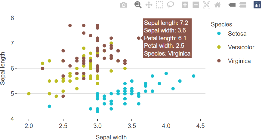

{ggblanket} provides access to all other geom_* arguments via ...

penguins %>%
  tidyr::drop_na(sex) %>%
  gg_smooth(
    x = flipper_length_mm,
    y = body_mass_g,
    col = sex,
    level = 0.99, #argument from geom_smooth
    col_legend_place = "t",
    col_title = "", 
    col_labels = snakecase::to_sentence_case
  )

{ggblanket} is useful for creating customised functions with your own defaults.

This is because the ... argument can allow you to access all arguments within the {ggblanket} gg_ function.

gg_point_custom <- function(data, x, y, col, 
                            size = 3, 
                            pal = pals::brewer.dark2(9), 
                            col_title = "", 
                            col_legend_place = "t",
                            ...) {
  data %>% 
    gg_point(x = {{ x }}, y = {{ y }}, col = {{col}}, 
             size = size, 
             pal = pal, 
             col_title = col_title, 
             col_legend_place = col_legend_place, 
             ...)
}

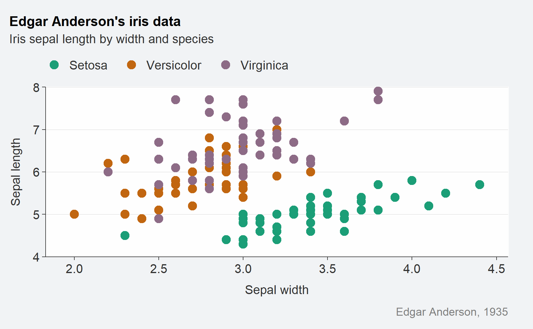
iris %>%
  mutate(Species = stringr::str_to_sentence(Species)) %>% 
  gg_point_custom(
    x = Sepal.Width,
    y = Sepal.Length,
    col = Species, 
    title = "Edgar Anderson's iris data",
    subtitle = "Iris sepal length by width and species",
    caption = "Edgar Anderson, 1935"
  )