![]()
![]()
![]()
ggnewscale tries to make it painless to use multiple scales in ggplot2. Although originally intended to use with colour and fill, it should work with any aes, such as shape, linetype and the rest. It’s very experimental, so use at your own risk!
For another way of defining multiple scales, you can also try relayer.
You can install ggnewscale from CRAN with:
Or the development version with:
If you use ggnewscale in a publication, I’ll be grateful if you cited it. To get the suggested citation for this (and any other R package) you can use:
citation("ggnewscale")
#>
#> To cite ggnewscale in publications use:
#>
#> Campitelli E (2022). _ggnewscale: Multiple Fill and Colour Scales in
#> 'ggplot2'_. doi: 10.5281/zenodo.2543762 (URL:
#> https://doi.org/10.5281/zenodo.2543762), R package version 0.4.7.
#>
#> A BibTeX entry for LaTeX users is
#>
#>   @Manual{R-ggnewscale,
#>     title = {ggnewscale: Multiple Fill and Colour Scales in 'ggplot2'},
#>     author = {Elio Campitelli},
#>     year = {2022},
#>     note = {R package version 0.4.7},
#>     doi = {10.5281/zenodo.2543762},
#>   }
If you use knitr, you can automate this with
And then add citations with @R-ggnewscale.
Click to see a list of some publications that have cited ggnewscale. Thanks!
[1] E. Akhil Prakash, T. Hromádková, T. Jabir, et al. “Dissemination of Multidrug Resistant Bacteria to the Polar Environment - Role of the Longest Migratory Bird Arctic Tern (Sterna Paradisaea)”. In: Science of The Total Environment (Dec. 31, 2021), p. 152727. ISSN: 0048-9697. DOI: 10.1016/j.scitotenv.2021.152727. <URL: https://www.sciencedirect.com/science/article/pii/S0048969721078062> (visited on 01/03/2022).
[2] R. AminiTabrizi, R. M. Wilson, J. D. Fudyma, et al. “Controls on Soil Organic Matter Degradation and Subsequent Greenhouse Gas Emissions Across a Permafrost Thaw Gradient in Northern Sweden”. In: Frontiers in Earth Science 8 (2020). ISSN: 2296-6463. DOI: 10.3389/feart.2020.557961. <URL: https://www.frontiersin.org/articles/10.3389/feart.2020.557961/full> (visited on 03/03/2021).
[3] X. Ding, K. Liu, Q. Yan, et al. “Sugar and Organic Acid Availability Modulate Soil Diazotroph Community Assembly and Species Co-Occurrence Patterns on the Tibetan Plateau”. In: Applied Microbiology and Biotechnology (Oct. 18, 2021). ISSN: 1432-0614. DOI: 10.1007/s00253-021-11629-9. <URL: https://doi.org/10.1007/s00253-021-11629-9> (visited on 10/21/2021).
[4] T. G. Drivas, A. Lucas, and M. D. Ritchie. “eQTpLot: A User-Friendly R Package for the Visualization of Colocalization between eQTL and GWAS Signals”. In: BioData Mining 14.1 (Jul. 17, 2021), p. 32. ISSN: 1756-0381. DOI: 10.1186/s13040-021-00267-6. <URL: https://doi.org/10.1186/s13040-021-00267-6> (visited on 07/21/2021).
[5] B. D. Golas, B. Goodell, and C. T. Webb. “Host Adaptation to Novel Pathogen Introduction: Predicting Conditions That Promote Evolutionary Rescue”. In: Ecology Letters 24.10 (2021), pp. 2238-2255. ISSN: 1461-0248. DOI: 10.1111/ele.13845. <URL: https://onlinelibrary.wiley.com/doi/abs/10.1111/ele.13845> (visited on 03/25/2022).
[6] M. C. Granovetter, L. Ettensohn, and M. Behrmann. “With Childhood Hemispherectomy, One Hemisphere Can Support—But Is Suboptimal for—Word and Face Recognition”. In: bioRxiv (Nov. 08, 2020), p. 2020.11.06.371823. DOI: 10.1101/2020.11.06.371823. <URL: https://www.biorxiv.org/content/10.1101/2020.11.06.371823v1> (visited on 03/03/2021).
[7] A. T. Hinsu, K. J. Panchal, R. J. Pandit, et al. “Characterizing Rhizosphere Microbiota of Peanut (Arachis Hypogaea L.) from Pre-Sowing to Post-Harvest of Crop under Field Conditions”. In: Scientific Reports 11.1 (1 Aug. 31, 2021), p. 17457. ISSN: 2045-2322. DOI: 10.1038/s41598-021-97071-3. <URL: https://www.nature.com/articles/s41598-021-97071-3> (visited on 09/06/2021).
[8] M. Jenckel, I. Smith, T. King, et al. “Distribution and Genetic Diversity of Hepatitis E Virus in Wild and Domestic Rabbits in Australia”. In: Pathogens 10.12 (12 Dec. 2021), p. 1637. DOI: 10.3390/pathogens10121637. <URL: https://www.mdpi.com/2076-0817/10/12/1637> (visited on 12/21/2021).
[9] M. Jung, D. Wells, J. Rusch, et al. “Unified Single-Cell Analysis of Testis Gene Regulation and Pathology in Five Mouse Strains”. In: eLife 8 (Jun. 25, 2019). Ed. by D. Bourc’his, P. J. Wittkopp and S. Lukassen, p. e43966. ISSN: 2050-084X. DOI: 10.7554/eLife.43966. <URL: https://doi.org/10.7554/eLife.43966> (visited on 03/03/2021).
[10] A. Lan, K. Kang, S. Tang, et al. “Fine-Scale Population Structure and Demographic History of Han Chinese Inferred from Haplotype Network of 111,000 Genomes”. In: bioRxiv (Jul. 04, 2020), p. 2020.07.03.166413. DOI: 10.1101/2020.07.03.166413. <URL: https://www.biorxiv.org/content/10.1101/2020.07.03.166413v2> (visited on 03/03/2021).
[11] Z. Lapp, R. Crawford, A. Miles-Jay, et al. “Regional Spread of blaNDM-1-containing Klebsiella Pneumoniae ST147 in Post-Acute Care Facilities”. In: Clinical Infectious Diseases (ciab457 May. 17, 2021). ISSN: 1058-4838. DOI: 10.1093/cid/ciab457. <URL: https://doi.org/10.1093/cid/ciab457> (visited on 05/21/2021).
[12] E. Merino Tejero, D. Lashgari, R. García-Valiente, et al. “Multiscale Modeling of Germinal Center Recapitulates the Temporal Transition From Memory B Cells to Plasma Cells Differentiation as Regulated by Antigen Affinity-Based Tfh Cell Help”. In: Frontiers in Immunology 11 (Feb. 05, 2021). ISSN: 1664-3224. DOI: 10.3389/fimmu.2020.620716. pmid: 33613551. <URL: https://www.ncbi.nlm.nih.gov/pmc/articles/PMC7892951/> (visited on 03/03/2021).
[13] G. Papacharalampous, H. Tyralis, S. M. Papalexiou, et al. “Global-Scale Massive Feature Extraction from Monthly Hydroclimatic Time Series: Statistical Characterizations, Spatial Patterns and Hydrological Similarity”. In: Science of The Total Environment 767 (May. 01, 2021), p. 144612. ISSN: 0048-9697. DOI: 10.1016/j.scitotenv.2020.144612. <URL: https://www.sciencedirect.com/science/article/pii/S0048969720381432> (visited on 03/03/2021).
[14] M. A. Prang, L. Zywucki, M. Körner, et al. “Differences in Sibling Cooperation in Presence and Absence of Parental Care in a Genus with Interspecific Variation in Offspring Dependence”. In: Evolution 76.2 (2022), pp. 320-331. ISSN: 1558-5646. DOI: 10.1111/evo.14414. <URL: https://onlinelibrary.wiley.com/doi/abs/10.1111/evo.14414> (visited on 03/25/2022).
[15] J. M. Quilty, A. E. Sikorska-Senoner, and D. Hah. “A Stochastic Conceptual-Data-Driven Approach for Improved Hydrological Simulations”. In: Environmental Modelling & Software (Jan. 16, 2022), p. 105326. ISSN: 1364-8152. DOI: 10.1016/j.envsoft.2022.105326. <URL: https://www.sciencedirect.com/science/article/pii/S1364815222000329> (visited on 01/19/2022).
[16] A. Rutz, M. Sorokina, J. Galgonek, et al. “Open Natural Products Research: Curation and Dissemination of Biological Occurrences of Chemical Structures through Wikidata”. In: bioRxiv (Mar. 01, 2021), p. 2021.02.28.433265. DOI: 10.1101/2021.02.28.433265. <URL: https://www.biorxiv.org/content/10.1101/2021.02.28.433265v1> (visited on 03/07/2021).
[17] M. R. Scharn, M. C. G. Brachmann, M. A. Patchett, et al. Vegetation Responses to 26 Years of Warming at Latnjajaure Field Station, Northern Sweden. https://doi.org/10.1139/AS-2020-0042. Apr. 01, 2021. <URL: https://cdnsciencepub.com/doi/abs/10.1139/AS-2020-0042> (visited on 04/05/2021).
[18] L. Seep, Z. Razaghi-Moghadam, and Z. Nikoloski. “Reaction Lumping in Metabolic Networks for Application with Thermodynamic Metabolic Flux Analysis”. In: Scientific Reports 11.1 (1 Apr. 20, 2021), p. 8544. ISSN: 2045-2322. DOI: 10.1038/s41598-021-87643-8. <URL: https://www.nature.com/articles/s41598-021-87643-8> (visited on 04/23/2021).
[19] O. Seppälä. “Spatial and Temporal Drivers of Soil Respiration in a Tundra Environment”. MA Thesis. FACULTY OF SCIENCE DEPARTMENT OF GEOSCIENCES AND GEOGRAPHY GEOGRAPHY: UNIVERSITY OF HELSINKI, 2020.
[20] L. Shah, C. A. Arnillas, and G. B. Arhonditsis. “Characterizing Temporal Trends of Meteorological Extremes in Southern and Central Ontario, Canada”. In: Weather and Climate Extremes (Jan. 25, 2022), p. 100411. ISSN: 2212-0947. DOI: 10.1016/j.wace.2022.100411. <URL: https://www.sciencedirect.com/science/article/pii/S2212094722000056> (visited on 01/29/2022).
[21] C. C. Smith, S. Entwistle, C. Willis, et al. “Landscape and Selection of Vaccine Epitopes in SARS-CoV-2”. In: bioRxiv (Jun. 04, 2020). DOI: 10.1101/2020.06.04.135004. pmid: 32577654. <URL: https://www.ncbi.nlm.nih.gov/pmc/articles/PMC7302209/> (visited on 03/03/2021).
[22] S. N. Thiede, E. S. Snitkin, W. Trick, et al. “Genomic Epidemiology Suggests Community Origins of Healthcare-Associated USA300 MRSA”. In: The Journal of Infectious Diseases (Feb. 16, 2022), p. jiac056. ISSN: 0022-1899. DOI: 10.1093/infdis/jiac056. <URL: https://doi.org/10.1093/infdis/jiac056> (visited on 02/26/2022).
[23] A. Torres-Espín, A. Chou, J. R. Huie, et al. “Reproducible Analysis of Disease Space via Principal Components Using the Novel R Package syndRomics”. In: eLife 10 (Jan. 14, 2021). Ed. by M. Zaidi and M. Barton, p. e61812. ISSN: 2050-084X. DOI: 10.7554/eLife.61812. <URL: https://doi.org/10.7554/eLife.61812> (visited on 03/03/2021).
[24] K. Tougeron and C. Iltis. “Impact of Heat Stress on the Fitness Outcomes of Symbiotic Infection in Aphids: A Meta-Analysis”. In: EcoEvoRxiv (Mar. 25, 2022). DOI: 10.32942/osf.io/nxdaw. <URL: https://ecoevorxiv.org/nxdaw/> (visited on 03/25/2022).
[25] L. Weidenauer and M. Quadroni. “Phosphorylation in the Charged Linker Modulates Interactions and Secretion of Hsp90β”. In: Cells 10.7 (7 Jul. 2021), p. 1701. DOI: 10.3390/cells10071701. <URL: https://www.mdpi.com/2073-4409/10/7/1701> (visited on 07/08/2021).
[26] D. Wendisch, O. Dietrich, T. Mari, et al. “SARS-CoV-2 Infection Triggers Profibrotic Macrophage Responses and Lung Fibrosis”. In: Cell (Nov. 27, 2021). ISSN: 0092-8674. DOI: 10.1016/j.cell.2021.11.033. <URL: https://www.sciencedirect.com/science/article/pii/S0092867421013830> (visited on 12/11/2021).
[27] R. J. Wright, M. G. I. Langille, and T. R. Walker. “Food or Just a Free Ride? A Meta-Analysis Reveals the Global Diversity of the Plastisphere”. In: The ISME Journal 15.3 (3 Mar. 2021), pp. 789-806. ISSN: 1751-7370. DOI: 10.1038/s41396-020-00814-9. <URL: https://www.nature.com/articles/s41396-020-00814-9> (visited on 03/03/2021).
[28] T. Wyenberg-Henzler, R. T. Patterson, and J. C. Mallon. “Ontogenetic Dietary Shifts in North American Hadrosaurids”. In: Cretaceous Research (Feb. 23, 2022), p. 105177. ISSN: 0195-6671. DOI: 10.1016/j.cretres.2022.105177. <URL: https://www.sciencedirect.com/science/article/pii/S0195667122000416> (visited on 02/26/2022).
[29] A. Yan, J. Butcher, D. Mack, et al. “Virome Sequencing of the Human Intestinal Mucosal–Luminal Interface”. In: Frontiers in Cellular and Infection Microbiology 10 (Oct. 22, 2020). ISSN: 2235-2988. DOI: 10.3389/fcimb.2020.582187. pmid: 33194818. <URL: https://www.ncbi.nlm.nih.gov/pmc/articles/PMC7642909/> (visited on 03/03/2021).
[30] P. Zannini, F. Frascaroli, J. Nascimbene, et al. “Sacred Natural Sites and Biodiversity Conservation: A Systematic Review”. In: Biodiversity and Conservation (Sep. 30, 2021). ISSN: 1572-9710. DOI: 10.1007/s10531-021-02296-3. <URL: https://doi.org/10.1007/s10531-021-02296-3> (visited on 10/04/2021).The main function is new_scale() and its aliases new_scale_color() and new_scale_fill(). When added to a plot, every geom added after them will use a different scale.
As an example, let’s overlay some measurements over a contour map of topography using the beloved volcano.
library(ggplot2)
library(ggnewscale)
# Equivalent to melt(volcano)
topography <- expand.grid(x = 1:nrow(volcano),
                          y = 1:ncol(volcano))
topography$z <- c(volcano)

# point measurements of something at a few locations
set.seed(42)
measurements <- data.frame(x = runif(30, 1, 80),
                           y = runif(30, 1, 60),
                           thing = rnorm(30))

ggplot(mapping = aes(x, y)) +
  geom_contour(data = topography, aes(z = z, color = stat(level))) +
  # Color scale for topography
  scale_color_viridis_c(option = "D") +
  # geoms below will use another color scale
  new_scale_color() +
  geom_point(data = measurements, size = 3, aes(color = thing)) +
  # Color scale applied to geoms added after new_scale_color()
  scale_color_viridis_c(option = "A")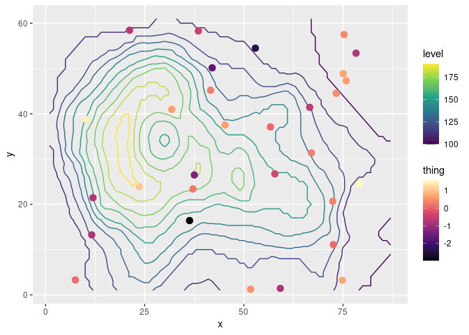
If you want to create new scales for other aes, you can call new_scale with the name of the aes. For example, use
to add multiple linetype scales.