![]()

ggsoccer provides a handful of functions that make it easy to plot soccer event data in R/ggplot2.
ggsoccer is available via CRAN:
Alternatively, you can download the development version from github like so:
![]()
The following example uses ggsoccer to solve a realistic problem: plotting a set of passes onto a soccer pitch.
pass_data <- data.frame(x = c(24, 18, 64, 78, 53),
                        y = c(43, 55, 88, 18, 44),
                        x2 = c(34, 44, 81, 85, 64),
                        y2 = c(40, 62, 89, 44, 28))

ggplot(pass_data) +
  annotate_pitch() +
  geom_segment(aes(x = x, y = y, xend = x2, yend = y2),
               arrow = arrow(length = unit(0.25, "cm"),
                             type = "closed")) +
  theme_pitch() +
  direction_label() +
  ggtitle("Simple passmap",
          "ggsoccer example")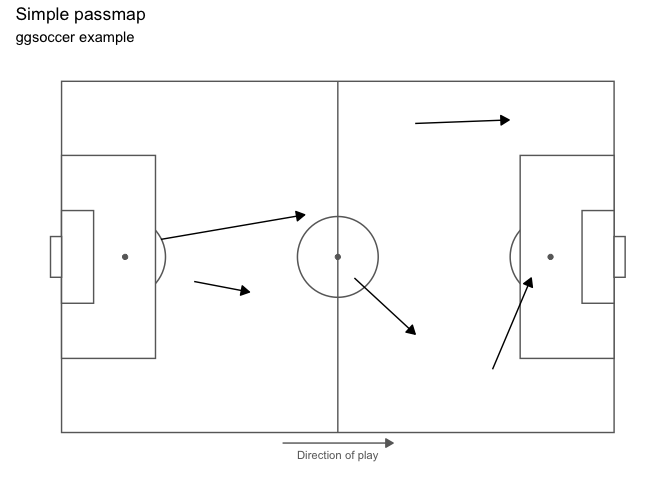
Because ggsoccer is implemented as ggplot layers, it makes customising a plot very easy. Here is a different example, plotting shots on a green pitch.
Note that by default, ggsoccer will display the whole pitch. To display a subsection of the pitch, simply set the plot limits as you would with any other ggplot2 plot. Here, we use the xlim and ylim arguments to coord_flip.
Because of the way coordinates get flipped, we must also reverse the y-axis to ensure that the orientation remains correct.
NOTE: Ordinarily, we would just do this with scale_y_reverse. However, due to a bug in ggplot2, this results in certain elements of the pitch (centre circle and penalty box arcs) failing to render. Instead, we can flip the y coordinates manually (100 - y in this case).
shots <- data.frame(x = c(90, 85, 82, 78, 83, 74, 94, 91),
                    y = c(43, 40, 52, 56, 44, 71, 60, 54))

ggplot(shots) +
  annotate_pitch(colour = "white",
                 fill   = "#7fc47f",
                 limits = FALSE) +
  geom_point(aes(x = x, y = 100 - y),
             colour = "black",
             fill = "chartreuse4",
             pch = 21,
             size = 2) +
  theme_pitch() +
  coord_flip(xlim = c(49, 101),
             ylim = c(-12, 112)) +
  ggtitle("Simple shotmap",
          "ggsoccer example")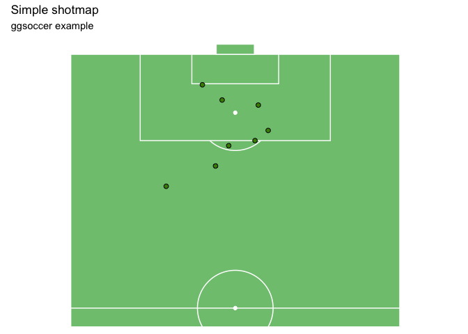
ggsoccer defaults to Opta’s 100x100 coordinate system. However, different data providers may use alternative coordinates.
ggsoccer provides support for a few data providers out of the box, as well as an interface for any custom coordinate system:
# ggsoccer enables you to rescale coordinates from one data provider to another, too
to_statsbomb <- rescale_coordinates(from = pitch_opta, to = pitch_statsbomb)

passes_rescaled <- data.frame(x  = to_statsbomb$x(pass_data$x),
                              y  = to_statsbomb$y(pass_data$y),
                              x2 = to_statsbomb$x(pass_data$x2),
                              y2 = to_statsbomb$y(pass_data$y2))

ggplot(passes_rescaled) +
  annotate_pitch(dimensions = pitch_statsbomb) +
  geom_segment(aes(x = x, y = y, xend = x2, yend = y2),
               colour = "coral",
               arrow = arrow(length = unit(0.25, "cm"),
                             type = "closed")) +
  theme_pitch() +
  direction_label(x_label = 60) +
  ggtitle("Simple passmap",
          "Statsbomb co-ordinates")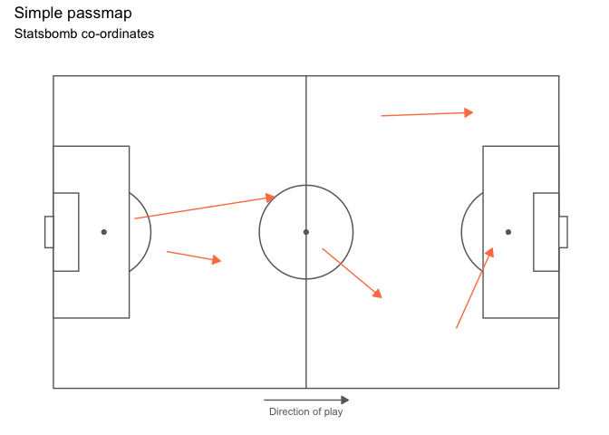
To plot data for a dataset not provided, ggsoccer just requires a pitch specification. This is a list containing the required pitch dimensions like so:
pitch_custom <- list(
  length = 150,
  width = 100,
  penalty_box_length = 25,
  penalty_box_width = 50,
  six_yard_box_length = 8,
  six_yard_box_width = 26,
  penalty_spot_distance = 16,
  goal_width = 12,
  origin_x = 0,
  origin_y = 0
)

ggplot() +
  annotate_pitch(dimensions = pitch_custom) +
  theme_pitch()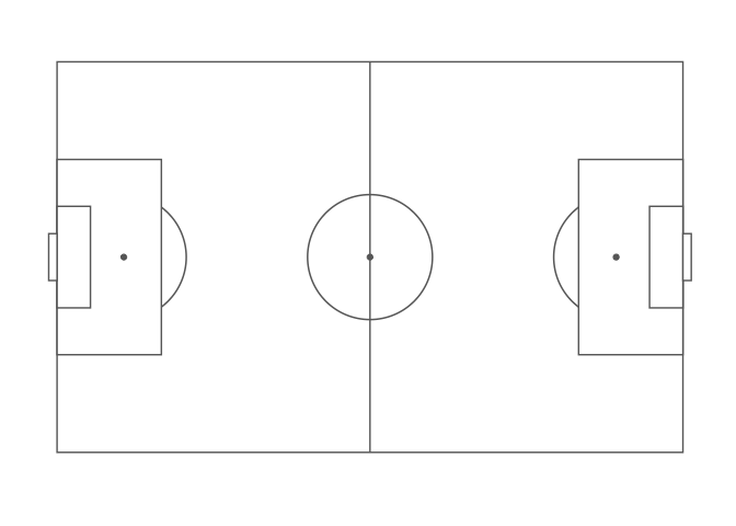
There are other packages that offer alternative pitch plotting options. Depending on your use case, you may want to check these out too: