The goal of healthyR.ts is to provide a consistent verb
framework for performing time series analysis and forecasting on both
administrative and clinical hospital data.
You can install the released version of healthyR.ts from CRAN with:
install.packages("healthyR.ts")And the development version from GitHub with:
# install.packages("devtools")
devtools::install_github("spsanderson/healthyR.ts")This is a basic example which shows you how to generate random walk data.
library(healthyR.ts)
library(ggplot2)

df <- ts_random_walk()

head(df)
#> # A tibble: 6 × 4
#>     run     x       y cum_y
#>   <dbl> <dbl>   <dbl> <dbl>
#> 1     1     1  0.0406 1041.
#> 2     1     2  0.114  1160.
#> 3     1     3 -0.0185 1138.
#> 4     1     4 -0.113  1010.
#> 5     1     5 -0.198   810.
#> 6     1     6 -0.170   672.
Now that the data has been generated, lets take a look at it.
df %>%
   ggplot(
       mapping = aes(
           x = x
           , y = cum_y
           , color = factor(run)
           , group = factor(run)
        )
    ) +
    geom_line(alpha = 0.8) +
    ts_random_walk_ggplot_layers(df)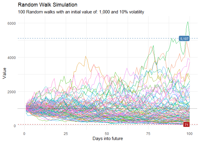
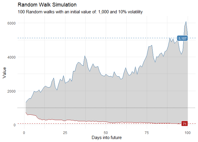
That is still pretty noisy, so lets see this in a different way. Lets clear this up a bit to make it easier to see the full range of the possible volatility of the random walks.
library(dplyr)
library(ggplot2)

df %>%
    group_by(x) %>%
    summarise(
        min_y = min(cum_y),
        max_y = max(cum_y)
    ) %>%
    ggplot(
        aes(x = x)
    ) +
    geom_line(aes(y = max_y), color = "steelblue") +
    geom_line(aes(y = min_y), color = "firebrick") +
    geom_ribbon(aes(ymin = min_y, ymax = max_y), alpha = 0.2) +
    ts_random_walk_ggplot_layers(df)