![]()


![]()
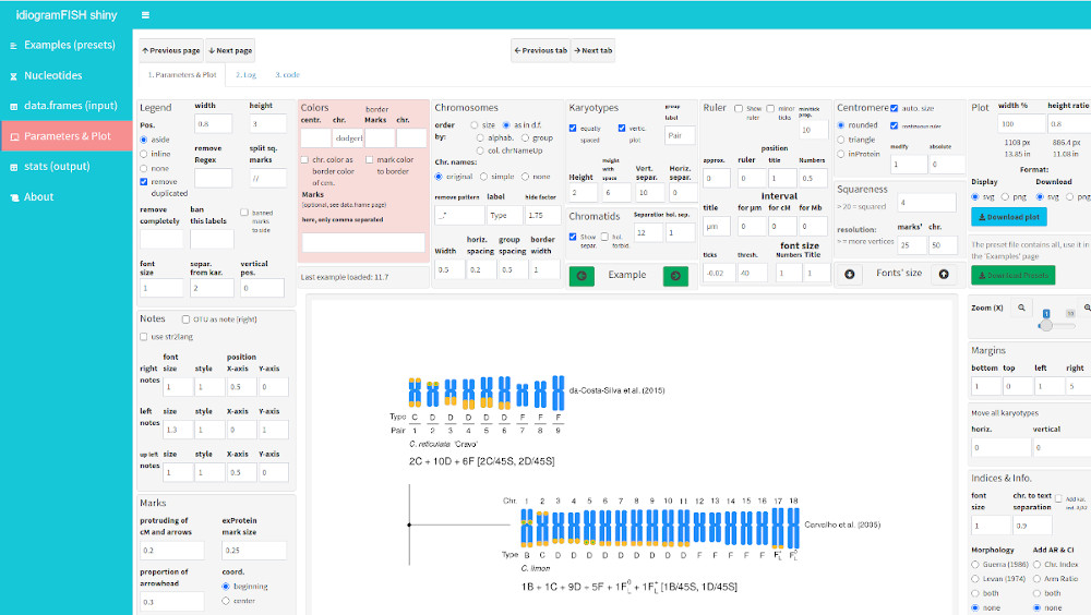
The goal of idiogramFISH functions or shiny-app is to plot karyotypes, plasmids and circular chr. having a set of data.frames for chromosome data and optionally marks’ data (Roa and PC Telles, 2021). Karyotypes can also be plotted in concentric circles.
It is possible to calculate also chromosome and karyotype indexes (Romero-Zarco, 1986; Watanabe et al., 1999) and classify chromosome morphology in the categories of Levan (1964), and Guerra (1986).
Six styles of marks are available: square (squareLeft), dots, cM (cMLeft), cenStyle, upArrow (downArrow), exProtein (inProtein) (column style in dfMarkColor data.frame); its legend (label) (parameter legend) can be drawn inline or to the right of karyotypes. Three styles of centromere are available: rounded, triangle and inProtein (cenFormat parameter). Chromosome regions (column chrRegion in dfMarkPos data.frame) for monocentrics are p, q, cen, pcen, qcen. The last three cannot accommodate most mark styles, but can be colored. The region w can be used both in monocentrics and holocentrics.
IdiogramFISH was written in R (R Core Team, 2019) and also uses crayon (Csárdi, 2017), tidyr (Wickham and Henry, 2020), plyr (Wickham, 2011) and dplyr packages (Wickham et al., 2019a). Documentation was written with R-packages roxygen2 (Wickham et al., 2018), usethis (Wickham and Bryan, 2019), bookdown (Xie, 2016), knitr (Xie, 2015), pkgdown (Wickham and Hesselberth, 2019), Rmarkdown (Xie et al., 2018), rvcheck (Yu, 2019a), badger (Yu, 2019b), kableExtra (Zhu, 2019), rmdformats (Barnier, 2020) and RCurl (Temple Lang and CRAN team, 2019). For some vignette figures, packages rentrez (Winter, 2017), phytools (Revell, 2012), ggtree (Yu et al., 2018), ggplot2 (Wickham, 2016) and ggpubr (Kassambara, 2019) were used.
In addition, the shiny app runBoard() uses shiny (Chang et al., 2021), shinydashboard (Chang and Borges Ribeiro, 2018), rhandsontable (Owen, 2018), gtools (Warnes et al., 2020) and rclipboard (Bihorel, 2021).
Windows users: To avoid installation of packages in OneDrive
To do that permanently: Search (magnifier) “environment variables” and set R_LIBS_USER to D:\R\lib (example)
Attention windows users, please install Rtools and git (compilation tools).
Vignettes (optional) use a lua filter, so you would need pandoc ver. > 2. and pandoc-citeproc or citeproc. RStudio comes with pandoc. rmarkdown::pandoc_version()
# This installs package devtools, necessary for installing the dev version
install.packages("devtools")

url <- "https://gitlab.com/ferroao/idiogramFISH"

# Packages for vignettes: (optional)
list.of.packages <- c(
    "knitr",
    "kableExtra",
    "rmdformats",
    "rmarkdown",
    "RCurl",
    "rvcheck",
    "badger",
    "rentrez"
    )
new.packages <- list.of.packages[!(list.of.packages %in% installed.packages()[,"Package"])]
if(length(new.packages)) install.packages(new.packages)

# Linux with vignettes and Windows
devtools::install_git(url = url,build_vignettes = TRUE, force=TRUE)

# Mac with vignettes
devtools::install_git(url = url, build_opts=c("--no-resave-data","--no-manual") )# clone repository:
git clone "https://gitlab.com/ferroao/idiogramFISH"
R CMD build idiogramFISH
# install
R CMD INSTALL idiogramFISH_*.tar.gz 

Online:

Launch vignettes from R for the installed version:
To cite idiogramFISH in publications, please use:
Roa F, Telles MPC (2021) idiogramFISH: Shiny app. Idiograms with Marks and Karyotype Indices, Universidade Federal de Goiás. Brazil. R-package. version 2.0.8 https://ferroao.gitlab.io/manualidiogramfish/. doi:10.5281/zenodo.3579417
To write citation to file:
Fernando Roa
Mariana PC Telles
For Shiny App in the cloud availability, please check this chapter in the online version https://ferroao.gitlab.io/idiogramfishhelppages
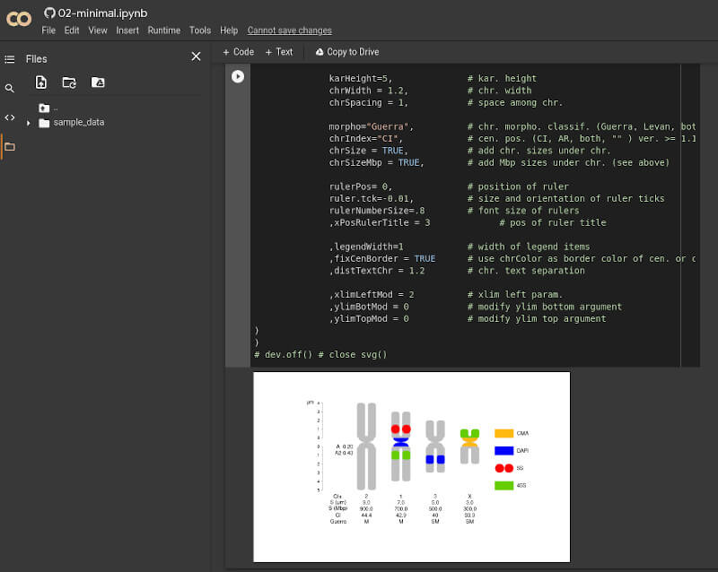
Each chapter has a jupyter version. A jupyter notebook seems an interactive vignette.
They are hosted in github
They can be accessed with google colab to work online.
Chapers can be accessed locally in your jupyter-lab or jupyter notebook
After installing jupyter, you can install the R kernel with:
Attention windows users, might require the last R version to plot correctly.
For Shiny App in the cloud availability, please check this chapter in the online version https://ferroao.gitlab.io/idiogramfishhelppages
Define your plotting window size with something like par(pin=c(10,6)), or with svg(), png(), etc. Add chromosome morphology according to Guerra (1986) or (Levan et al., 1964)
library(idiogramFISH)

data(dfOfChrSize) # chromsome data
data(dfMarkColor) # mark general data
data(dfOfMarks2)  # mark position data (inc. cen.)

dfOfMarks2[which(dfOfMarks2$markName=="5S"),]$markSize<-0.8 # modif. of mark size

# column Mbp not for plotting purposes
dfOfChrSize$Mbp<-(dfOfChrSize$shortArmSize+dfOfChrSize$longArmSize)*100

opar <- par(no.readonly = TRUE)      # make a copy of current settings if you want to restore them later
#par(opar) # recover par

par(mar=rep(0,4))

plotIdiograms(dfChrSize=dfOfChrSize,    # data.frame of chr. size
              dfMarkColor=dfMarkColor,  # d.f of mark style <- Optional
              dfMarkPos=dfOfMarks2,     # df of mark positions (includes cen. marks)

              karHeight=5,              # kar. height
              chrWidth = 1.2,           # chr. width
              chrSpacing = 1,           # space among chr.

              morpho="Guerra",          # chr. morpho. classif. (Guerra, Levan, both, "" ) ver. >= 1.12 only
              chrIndex="CI",            # cen. pos. (CI, AR, both, "" ) ver. >= 1.12 only
              chrSize = TRUE,           # add chr. sizes under chr.
              chrSizeMbp = TRUE,        # add Mbp sizes under chr. (see above)

              rulerPos= 0,              # position of ruler
              ruler.tck=-0.01,          # size and orientation of ruler ticks
              rulerNumberSize=.8        # font size of rulers
              ,xPosRulerTitle = 3             # ruler units (title) pos.

              ,legendWidth=1            # width of legend items
              ,fixCenBorder = TRUE      # use chrColor as border color of cen. or cen. marks
              ,distTextChr = 1.2        # chr. text separation

              ,xlimLeftMod = 2          # xlim left param.
              ,ylimBotMod = 0           # modify ylim bottom argument
              ,ylimTopMod = 0           # modify ylim top argument
); # dev.off() # close svg()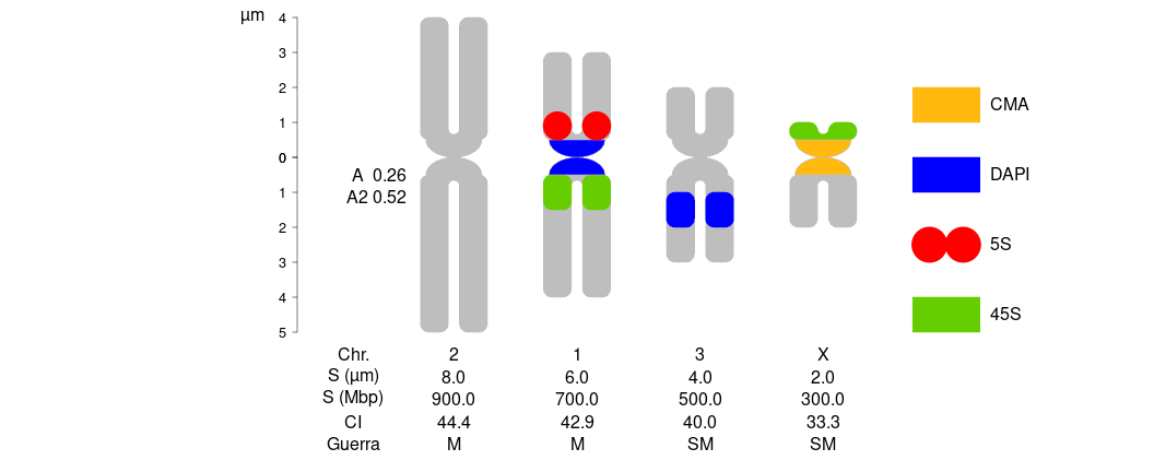
dfOfChrSize| chrName | shortArmSize | longArmSize | Mbp |
|---|---|---|---|
| 1 | 3 | 4 | 700 |
| 2 | 4 | 5 | 900 |
| 3 | 2 | 3 | 500 |
| X | 1 | 2 | 300 |
dfMarkColor| markName | markColor | style |
|---|---|---|
| 5S | red | dots |
| 45S | chartreuse3 | square |
| DAPI | blue | square |
| CMA | darkgoldenrod1 | square |
p, q and w marks can have empty columns markDistCen and markSize since v. 1.9.1 to plot whole arms (p, q) and whole chr. w.
dfOfMarks2| chrName | markName | chrRegion | markSize | markDistCen |
|---|---|---|---|---|
| 1 | 5S | p | 0.8 | 0.5 |
| 1 | 45S | q | 1.0 | 0.5 |
| X | 45S | p | NA | NA |
| 3 | DAPI | q | 1.0 | 1.0 |
| 1 | DAPI | cen | NA | NA |
| X | CMA | cen | NA | NA |
library(idiogramFISH)

# column Mbp not for plotting purposes
dfChrSizeHolo$Mbp<-dfChrSizeHolo$chrSize*100

# svg("testing.svg",width=14,height=8 )
par(mar = c(0, 0, 0, 0), omi=rep(0,4) )

plotIdiograms(dfChrSize  =dfChrSizeHolo, # data.frame of chr. size
              dfMarkColor=dfMarkColor,   # df of mark style
              dfMarkPos  =dfMarkPosHolo, # df of mark positions

              addOTUName=FALSE,        # do not add OTU names
              distTextChr = 1,         # chr. name distance to chr.
              chrSize = TRUE,          # show chr. size under chr.
              chrSizeMbp = TRUE,       # show chr. size in Mbp under chr. requires Mbp column

              rulerPos=-.4,            # position of ruler
              rulerNumberPos=.9,       # position of numbers of rulers
              xPosRulerTitle= 4.5            # ruler units (title) horizon. pos.

              ,xlimLeftMod=2           # modify xlim left argument of plot
              ,ylimBotMod=.2           # modify ylim bottom argument of plot
              ,legendHeight=.5         # height of legend labels
              ,legendWidth = 1.2       # width of legend labels
              ,xModifier = 20        # separ. among chromatids
); # dev.off() # close svg()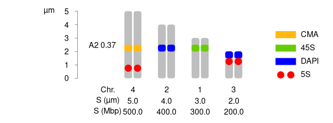
dfChrSizeHolo| chrName | chrSize | Mbp |
|---|---|---|
| 1 | 3 | 300 |
| 2 | 4 | 400 |
| 3 | 2 | 200 |
| 4 | 5 | 500 |
dfMarkColor| markName | markColor | style |
|---|---|---|
| 5S | red | dots |
| 45S | chartreuse3 | square |
| DAPI | blue | square |
| CMA | darkgoldenrod1 | square |
dfMarkPosHolo| chrName | markName | markPos | markSize |
|---|---|---|---|
| 3 | 5S | 1.0 | 0.5 |
| 3 | DAPI | 1.5 | 0.5 |
| 1 | 45S | 2.0 | 0.5 |
| 2 | DAPI | 2.0 | 0.5 |
| 4 | CMA | 2.0 | 0.5 |
| 4 | 5S | 0.5 | 0.5 |
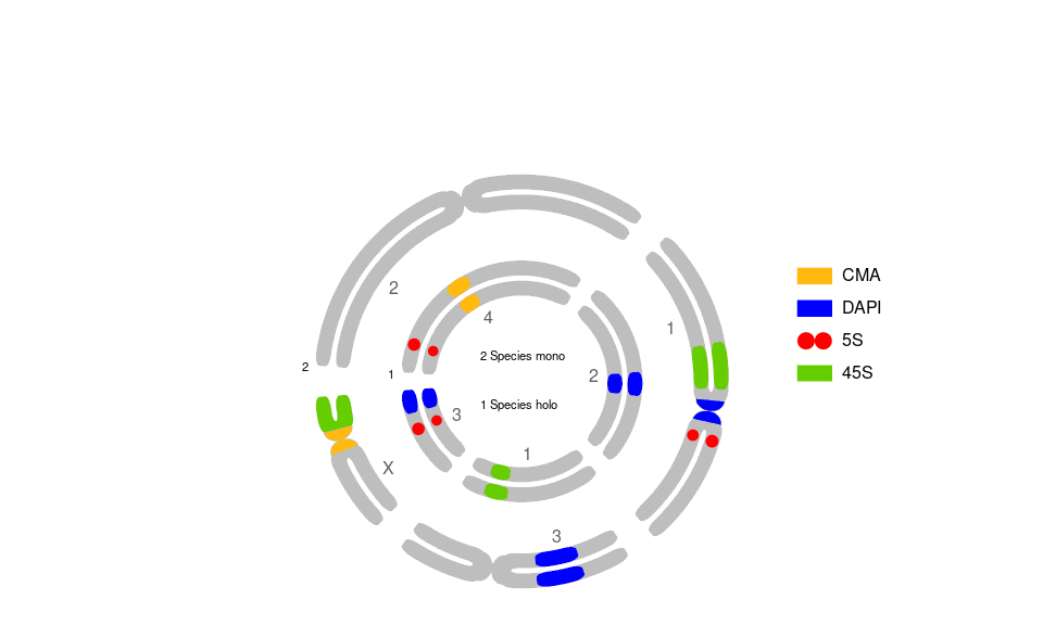
See vignettes for a circular version.
Merge data.frames with plyr (Wickham, 2011)
# chromsome data, if only 1 species, column OTU is optional
require(plyr)
dfOfChrSize$OTU   <- "Species mono"
dfChrSizeHolo$OTU <- "Species holo"

monoholoCS <- plyr::rbind.fill(dfOfChrSize,dfChrSizeHolo)

dfOfMarks2$OTU     <-"Species mono"
dfMarkPosHolo$OTU <-"Species holo"

monoholoMarks <- plyr::rbind.fill(dfOfMarks2,dfMarkPosHolo)
monoholoMarks[which(monoholoMarks$markName=="5S"),]$markSize<-.25
monoholoMarks
   chrName markName chrRegion markSize markDistCen          OTU markPos
1        1       5S         p     0.25         0.5 Species mono      NA
2        1      45S         q     1.00         0.5 Species mono      NA
3        X      45S         p       NA          NA Species mono      NA
4        3     DAPI         q     1.00         1.0 Species mono      NA
5        1     DAPI       cen       NA          NA Species mono      NA
6        X      CMA       cen       NA          NA Species mono      NA
7        3       5S      <NA>     0.25          NA Species holo     1.0
8        3     DAPI      <NA>     0.50          NA Species holo     1.5
9        1      45S      <NA>     0.50          NA Species holo     2.0
10       2     DAPI      <NA>     0.50          NA Species holo     2.0
11       4      CMA      <NA>     0.50          NA Species holo     2.0
12 4 5S <NA> 0.25 NA Species holo 0.5library(idiogramFISH)
# svg("testing.svg",width=10,height=6 )
par(mar=rep(0,4))
plotIdiograms(dfChrSize = monoholoCS, # data.frame of chr. size
dfMarkColor= dfMarkColor, # df of mark style
dfMarkPos = monoholoMarks,# df of mark positions, includes cen. marks
chrSize = TRUE, # show chr. size under chr.
squareness = 4, # vertices squareness
addOTUName = TRUE, # add OTU names
OTUTextSize = .7, # font size of OTU
distTextChr = 0.7, # separ. among chr. and text and among chr. name and indices
karHeiSpace = 4, # karyotype height inc. spacing
karIndexPos = .2, # move karyotype index
legendHeight= 1, # height of legend labels
legendWidth = 1, # width of legend labels
fixCenBorder = TRUE, # use chrColor as border color of cen. or cen. marks
rulerPos= 0, # position of ruler
ruler.tck=-0.02, # size and orientation of ruler ticks
rulerNumberPos=.9, # position of numbers of rulers
xPosRulerTitle= 4, # ruler units (title) pos.
xlimLeftMod=1, # modify xlim left argument of plot
xlimRightMod=3, # modify xlim right argument of plot
ylimBotMod= .2 # modify ylim bottom argument of plot
,chromatids=TRUE # do not show separ. chromatids
,autoCenSize=FALSE
,centromereSize = 0.5
# for Circular Plot, add:
# ,useOneDot=FALSE # two dots
# ,circularPlot = TRUE # circularPlot
# ,shrinkFactor = .9 # percentage 1 = 100% of circle with chr.
# ,circleCenter = 3 # X coordinate of circleCenter (affects legend pos.)
# ,chrLabelSpacing = .9 # chr. names spacing
# ,OTUsrt = 0 # angle for OTU name (or number)
# ,OTUplacing = "number" # Use number and legend instead of name
# ,OTULabelSpacerx = -0.6 # modify position of OTU label, when OTUplacing="number" or "simple"
# ,OTUlegendHeight = 1.5 # space among OTU names when in legend - OTUplacing
# ,separFactor = 0.75 # alter separ. of kar.
); # dev.off() # close svg()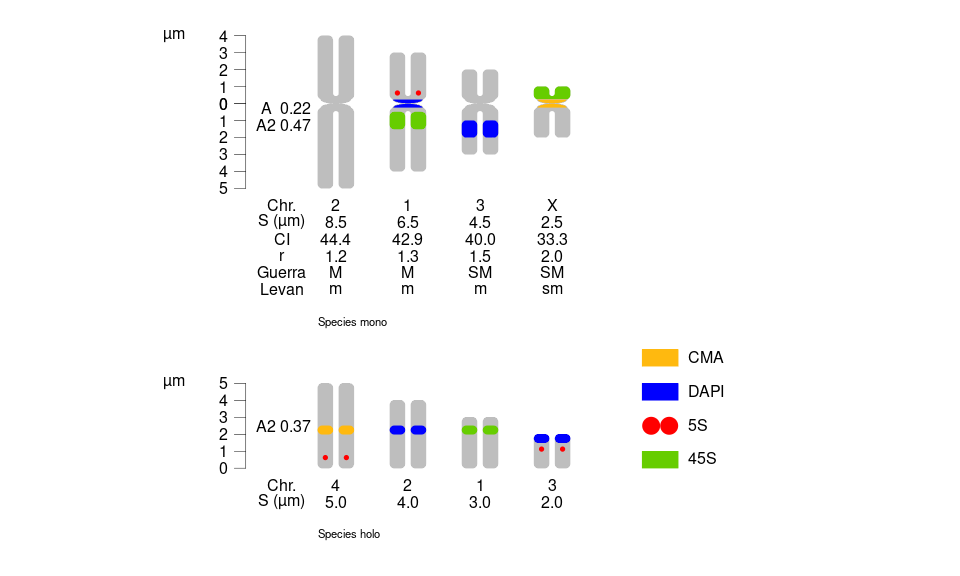
Guerra M. 1986. Reviewing the chromosome nomenclature of Levan et al. Brazilian Journal of Genetics, 9(4): 741–743
Levan A, Fredga K, Sandberg AA. 1964. Nomenclature for centromeric position on chromosomes Hereditas, 52(2): 201–220. https://onlinelibrary.wiley.com/doi/abs/10.1111/j.1601-5223.1964.tb01953.x
Romero-Zarco C. 1986. A new method for estimating karyotype asymmetry Taxon, 35(3): 526–530. https://onlinelibrary.wiley.com/doi/abs/10.2307/1221906
Watanabe K, Yahara T, Denda T, Kosuge K. 1999. Chromosomal evolution in the genus Brachyscome (Asteraceae, Astereae): statistical tests regarding correlation between changes in karyotype and habit using phylogenetic information Journal of Plant Research, 112: 145–161. https://link.springer.com/article/10.1007/PL00013869
Csárdi G. 2017. Crayon: Colored terminal output. R package version 1.3.4. https://CRAN.R-project.org/package=crayon
Kassambara A. 2019. Ggpubr: ’ggplot2’ based publication ready plots. R package version 0.2.3. https://CRAN.R-project.org/package=ggpubr
R Core Team. 2019. R: A language and environment for statistical computing R Foundation for Statistical Computing, Vienna, Austria. https://www.R-project.org/
Revell LJ. 2012. Phytools: An r package for phylogenetic comparative biology (and other things). Methods in Ecology and Evolution, 3: 217–223. https://besjournals.onlinelibrary.wiley.com/doi/10.1111/j.2041-210X.2011.00169.x
Roa F, PC Telles M. 2021. idiogramFISH: Shiny app. Idiograms with marks and karyotype indices Universidade Federal de Goiás, UFG, Goiânia. R-package. version 2.0.0. https://doi.org/10.5281/zenodo.3579417. https://ferroao.gitlab.io/manualidiogramfish/
Wickham H. 2011. The split-apply-combine strategy for data analysis Journal of Statistical Software, 40(1): 1–29. https://www.jstatsoft.org/article/view/v040i01
Wickham H. 2016. ggplot2: Elegant graphics for data analysis Springer-Verlag New York. https://ggplot2.tidyverse.org
Wickham H, François R, Henry L, Müller K. 2019a. Dplyr: A grammar of data manipulation. R package version 0.8.3. https://CRAN.R-project.org/package=dplyr
Wickham H, Henry L. 2020. Tidyr: Tidy messy data. R package version 1.0.2. https://CRAN.R-project.org/package=tidyr
Wickham H, Hester J, Chang W. 2019b. Devtools: Tools to make developing r packages easier. R package version 2.2.1. https://CRAN.R-project.org/package=devtools
Winter DJ. 2017. rentrez: An r package for the NCBI eUtils API The R Journal, 9: 520–526
Yu G, Lam TT-Y, Zhu H, Guan Y. 2018. Two methods for mapping and visualizing associated data on phylogeny using ggtree. Molecular Biology and Evolution, 35: 3041–3043. https://doi.org/10.1093/molbev/msy194. https://academic.oup.com/mbe/article/35/12/3041/5142656
Bihorel S. 2021. Rclipboard: Shiny/r wrapper for clipboard.js. R package version 0.1.3. https://github.com/sbihorel/rclipboard/
Chang W, Borges Ribeiro B. 2018. Shinydashboard: Create dashboards with shiny. R package version 0.7.1. http://rstudio.github.io/shinydashboard/
Chang W, Cheng J, Allaire J, Sievert C, Schloerke B, Xie Y, Allen J, McPherson J, Dipert A, Borges B. 2021. Shiny: Web application framework for r. R package version 1.6.0. https://shiny.rstudio.com/
Owen J. 2018. Rhandsontable: Interface to the handsontable.js library. R package version 0.3.7. http://jrowen.github.io/rhandsontable/
Warnes GR, Bolker B, Lumley T. 2020. Gtools: Various r programming tools. R package version 3.8.2. https://github.com/r-gregmisc/gtools
Barnier J. 2020. Rmdformats: HTML output formats and templates for ’rmarkdown’ documents. R package version 0.3.7. https://CRAN.R-project.org/package=rmdformats
Temple Lang D, CRAN team the. 2019. RCurl: General network (HTTP/FTP/…) Client interface for r. R package version 1.95-4.12. https://CRAN.R-project.org/package=RCurl
Wickham H, Bryan J. 2019. Usethis: Automate package and project setup. R package version 1.5.1. https://CRAN.R-project.org/package=usethis
Wickham H, Danenberg P, Eugster M. 2018. roxygen2: In-line documentation for r. R package version 6.1.1. https://CRAN.R-project.org/package=roxygen2
Wickham H, Hesselberth J. 2019. Pkgdown: Make static HTML documentation for a package. R package version 1.4.1. https://CRAN.R-project.org/package=pkgdown
Xie Y. 2015. Dynamic documents with R and knitr Chapman; Hall/CRC, Boca Raton, Florida. ISBN 978-1498716963. https://yihui.org/knitr/
Xie Y. 2016. Bookdown: Authoring books and technical documents with R markdown Chapman; Hall/CRC, Boca Raton, Florida. ISBN 978-1138700109. https://github.com/rstudio/bookdown
Xie Y, Allaire JJ, Grolemund G. 2018. R markdown: The definitive guide Chapman; Hall/CRC, Boca Raton, Florida. ISBN 9781138359338. https://bookdown.org/yihui/rmarkdown
Yu G. 2019b. Badger: Badge for r package. R package version 0.0.6. https://CRAN.R-project.org/package=badger
Yu G. 2019a. Rvcheck: R/package version check. R package version 0.1.6. https://CRAN.R-project.org/package=rvcheck
Zhu H. 2019. kableExtra: Construct complex table with ’kable’ and pipe syntax. R package version 1.1.0. https://CRAN.R-project.org/package=kableExtra