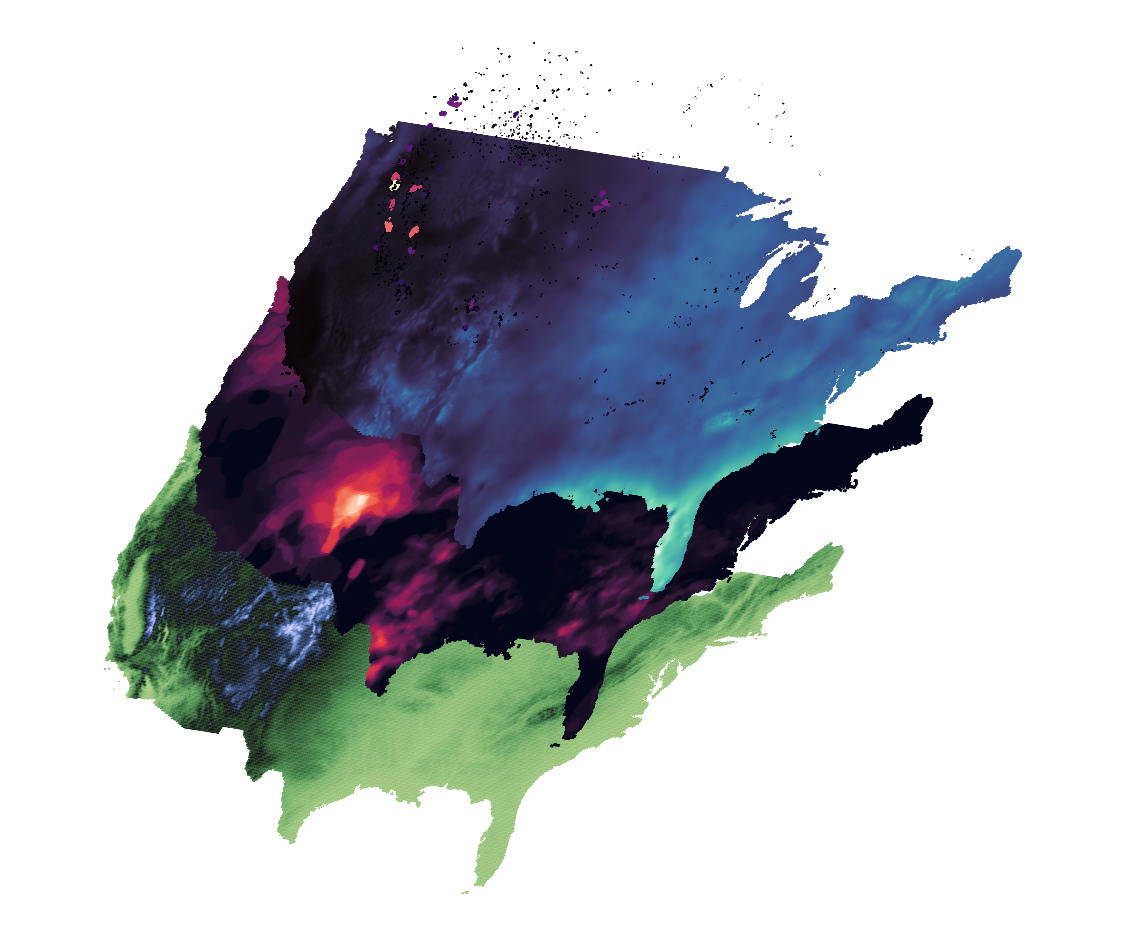
The goal of layer is to simplify the whole process of creating stacked tilted maps, that are often used in scientific publications to show different environmental layers for a geographical region. Tilting maps and layering them allows to easily draw visual correlations between these environmental layers.
Something in the line of:
You can install the development version of layer from GitHub with:
This is a basic example which shows you how to solve a common problem:
library(layer)

tilt_landscape_1 <- tilt_map(landscape_1)
#> Loading required package: raster
#> Loading required package: sp
tilt_landscape_2 <- tilt_map(landscape_2, x_shift = 50, y_shift = 50)
tilt_landscape_3 <- tilt_map(landscape_3, x_shift = 100, y_shift = 100)
tilt_landscape_points <- tilt_map(landscape_points, x_shift = 150, y_shift = 150)

map_list <- list(tilt_landscape_1, tilt_landscape_2, tilt_landscape_3, tilt_landscape_points)

plot_tiltedmaps(map_list,
                layer = c("value", "value", "value", NA),
                palette = c("bilbao", "mako", "rocket", "turbo"),
                color = "grey40")
#> Warning in if (is.na(layer)) layer <- "value": the condition has length > 1 and
#> only the first element will be used
Some more realistic looking data (DEM, drought and precipitation for continental USA):
tilt_landscape_1 <- tilt_map(dem_usa, y_tilt = 3)
tilt_landscape_2 <- tilt_map(drought_usa, y_tilt = 3, x_shift = 15, y_shift = 25)
tilt_landscape_3 <- tilt_map(prec_usa,y_tilt = 3,  x_shift = 30, y_shift = 50)
tilt_landscape_4 <- tilt_map(fire_usa,y_tilt = 3, x_shift = 45, y_shift = 65)

map_list <- list(tilt_landscape_1, tilt_landscape_2, tilt_landscape_3, tilt_landscape_4)

plot_tiltedmaps(map_list, palette =c("tofino", "rocket", "mako", "magma"), direction = c(-1, 1, 1, 1)) 
Please note that the layer project is released with a Contributor Code of Conduct. By contributing to this project, you agree to abide by its terms.