The goal of mapfit is to estimate parameters of phase-type distribution (PH) and Markovian arrival process (MAP). PH/MAP fitting is required in the analysis of non-Markovian models involving general distributions. By replacing general distributions with estimated PH/MAP, we have approximate the non-Markovian models with continuous-time Markov chains (CTMCs). Our tool offers
These features help us to analyze non-Markovian models with phase expansion.
# Install devtools from CRAN
install.packages("mapfit")

# Or the development version from GitHub:
# install.packages("devtools")
devtools::install_github("okamumu/mapfit")
PH distribution is defined as the time to absorption in a
time-homogeneous CTMC with an absorbing state. The p.d.f. and cumulative
distribution function (c.d.f.) are mathematically given as the
expressions using matrix exponential. Let and
denote a probability
(row) vector for determining an initial state and an infinitesimal
generator for transient states, respectively. Since the c.d.f. is given
by the probability that the current state of underlying CTMC has already
been absorbed, the c.d.f. of PH distribution is given by
[ F(x) = 1 - \boldsymbol{\alpha} \exp(\boldsymbol{Q} x) \boldsymbol{1},](https://latex.codecogs.com/png.image?%5Cdpi%7B110%7D&space;%5Cbg_white&space;%0AF%28x%29%20%3D%201%20-%20%5Cboldsymbol%7B%5Calpha%7D%20%5Cexp%28%5Cboldsymbol%7BQ%7D%20x%29%20%5Cboldsymbol%7B1%7D%2C%0A ” F(x) = 1 - ( x) , “)
where is a column vector whose
entries are 1. Also the p.d.f. can be obtained by taking the first
derivative of the c.d.f.;
[ f(x) = \boldsymbol{\alpha} \exp(\boldsymbol{Q} x) \boldsymbol{\xi},](https://latex.codecogs.com/png.image?%5Cdpi%7B110%7D&space;%5Cbg_white&space;%0Af%28x%29%20%3D%20%5Cboldsymbol%7B%5Calpha%7D%20%5Cexp%28%5Cboldsymbol%7BQ%7D%20x%29%20%5Cboldsymbol%7B%5Cxi%7D%2C%0A ” f(x) = ( x) , “)
where .
The purpose of PH fitting is to determine PH parameters and
so that the estimated PH
distribution fits to observed data. There are two different approaches;
MM (moment match) method and MLE (maximum likelihood estimation). The MM
method is to find PH parameters whose first few moments match to the
moments from empirical data or distribution functions. On the other
hand, MLE is to find PH parameters maximizing the likelihood
(probability) of which the data is drawn from the model as a sample.
The parameter estimation algorithm generally depends on data forms to be used. mapfit deals with several kinds of data in PH fitting; point data, weighted point data, grouped data, grouped data with missing values and truncated data. The point data consists of independent and identically-distributed (IID) random samples.
| Sample No. | Time |
|---|---|
| 1 | 10.0 |
| 2 | 1.4 |
| … | … |
| 100 | 51.0 |
The above table shows an example of point data for a hundred IID samples. The weighted point data is the point data in which all points have their own weights. The weighted point data is used for numerical integration of a density function in our tool. The grouped data consists of break points and counts. For each of two successive break points, the number of samples is counted as a bin. This is equivalent to the data format to draw a histogram.
The grouped data with missing values allows us to use the grouped
data in which several counts are unknown (missing). In the tool, missing
counts are expressed by NA. Also, in the truncated data,
several samples are truncated at a point before their observations
(right censored data). The truncated data can be represented as the
number of samples in a specific interval from the point to infinity in
the context of grouped data.
| Time interval | Counts |
|---|---|
| [0, 10] | 1 |
| [10, 20] | NA |
| [20, 30] | 4 |
| [30, 40] | 10 |
| [40, 50] | NA |
| [50, 60] | 30 |
| [60, 70] | 10 |
| [70, 80] | 12 |
| [80, 90] | 4 |
| [90, 100] | 0 |
| [100, Inf) | 5 |
The above table shows an example of the grouped data on break points 0, 10, 20, …, 100 where the data has missing values at the intervals [10,20] and [40,50]. Furthermore, the last 5 samples are truncated at 100.
| Time interval | Counts |
|---|---|
| [0, 10] | 1 |
| [10, 20] | NA |
| [20, 30] | 4 |
| [30, 40] | 10 |
| [40, 50] | NA |
| [50, 60] | 30 |
| [60, 70] | 10 |
| [70, 80] | 12 |
| [80, 90] | 4 |
| [90, 100] | 0 |
| [100, Inf) | NA |
On the other hand, the aboe table shows an example of another grouped data. In this case, several samples are truncated at 100 but we do not know the exact number of truncated samples.
PH distributions are classified to sub-classes by the structure of
and
, and the parameter
estimation algorithms depend on the class of PH distribution. The tool
deals with the following classes of PH distribution:
The parameters of ph class are ,
and
, which are defined as
members, called slots, of S4 class in R. To represent the
matrix
, we use
Matrix package which is an external package of R. The slots
of cf1 class are inherited from the ph class.
In addition to inherited slots, cf1 has a slot
rate to store the absolute values of diagonal elements of
. The
herlang
class has the slots for the mixed ratio, shape parameters of Erlang
components, rate parameters of Erlang components. Both of
cf1 and herlang classes can be transformed to
ph class by using `as’ method of R.
The R functions for PH parameter estimation are;
phfit.point: MLEs for general PH, CF1 and hyper-Erlang
distribution from point and weighted point data. The estimation
algorithms for general PH and CF1 are the EM algorithms proposed in [1].
The algorithm for hyper-Erlang distribution is the EM algorithm with
shape parameter selection described in [2,3].phfit.group: MLEs for general PH, CF1 and hyper-Erlang
distribution from grouped and truncated data. The estimation algorithms
for general PH and CF1 are the EM algorithms proposed in [4]. The
algorithm for hyper-Erlang distribution is the EM algorithm with shape
parameter selection, which is originally developed as an extension of
[2,3].phfit.density: MLEs for general PH, CF1 and
hyper-Erlang distribution from a density function defined on the
positive domain [0, Inf). The function phfit.density calls
phfit.point after making weighted point data. The weighted
point data is generated by numerical quadrature. In the tool, the
numerical quadrature is performed with a double exponential (DE)
formula.phfit.3mom: MM methods for acyclic PH distribution with
the first three moments [5,6].The functions phfit.point, phfit.group and
phfit.density select an appropriate algorithm depending on
the class of a given PH distribution. These functions return a list
including the estimated model (ph, cf1 or
herlang), the maximum log-likelihood (llf), Akaike
information criterion (aic) and other statistics of the estimation
algorithm. Also, the function phfit.3mom returns a
ph class whose first three moments match to the given three
moments.
Here we introduce examples of the usage of PH fitting based on IID samples from Weibull distribution. At first, we load the mapfit package and generate IID samples from a Weibull distribution:
library(mapfit)

RNGkind(kind = "Mersenne-Twister")
set.seed(1234)
wsample <- rweibull(100, shape=2, scale=1)
wsample is set to a vector including a hundred IID
samples generated from Weibull distribution with scale parameter 1 and
shape parameter 2. set.seed(1234) means determing the seed
of random numbers.
wsample
#>   [1] 1.47450394 0.68871906 0.70390766 0.68745901 0.38698715 0.66768398
#>   [7] 2.15798755 1.20774494 0.63744792 0.81550201 0.60487388 0.77911210
#>  [13] 1.12394405 0.28223484 1.10901777 0.42140013 1.11847354 1.14942511
#>  [19] 1.29542664 1.20832306 1.07241633 1.09317655 1.35593576 1.79415102
#>  [25] 1.23272029 0.45823831 0.80189104 0.29867185 0.42977942 1.75616647
#>  [31] 0.88603717 1.15209430 1.09019210 0.82379560 1.30718279 0.52428076
#>  [37] 1.26618210 1.16260990 0.08877248 0.46259605 0.76928163 0.66055079
#>  [43] 1.07949774 0.68927927 1.05326127 0.83015673 0.62445527 0.85066119
#>  [49] 1.18780419 0.51698994 1.61451826 1.08267929 0.57645512 0.82710123
#>  [55] 1.37015479 0.82783512 0.83982074 0.53486736 1.32097400 0.40547750
#>  [61] 0.38107465 1.78142911 1.07157783 2.07043978 1.19632106 0.58944015
#>  [67] 1.08505663 0.82231170 1.72143270 0.75610263 1.45189672 0.33667780
#>  [73] 2.05544853 0.49443698 1.55189411 0.80962054 0.97796650 1.63049390
#>  [79] 1.06650011 0.63460678 0.27649350 0.86658386 1.39556590 0.77994249
#>  [85] 1.27622488 0.32701528 0.97102624 1.08091533 1.35366256 0.33107018
#>  [91] 1.33917815 0.32386549 1.41750912 1.42403682 1.50035348 0.81868450
#>  [97] 1.09695465 1.90327589 1.08273771 0.54611792
Based on the point data, we can estimate PH parameters. Here we obtain the estimated parameters for general PH with 5 states, CF1 with 5 states and the hyper-Erlang with 5 states by the following commands, respectively;
## phfit with GPH
phfit.point(ph=ph(5), x=wsample)
#>
#> Maximum LLF: -59.436973
#> AIC: 176.873945
#> Iteration:  2000 / 2000
#> Computation time (user): 0.924000
#> Convergence: FALSE
#> Error (abs): 2.658070e-05 (tolerance Inf)
#> Error (rel): 4.472080e-07 (tolerance 1.490116e-08)
#>
#> Size : 5
#> Initial :  8.354082e-11 0.9958273 0.0006050049 0.003567682 9.063406e-95
#> Exit    :  0.1179994 3.90902e-93 6.464486e-06 0.05132675 4.831416
#> Infinitesimal generator :
#> 5 x 5 sparse Matrix of class "dgCMatrix"
#>
#> [1,] -4.871469e+00  4.471403e-144   1.628003e-66  5.694646e-18  4.75347004
#> [2,]  6.303324e-02  -4.830687e+00   4.592402e+00  8.763450e-03  0.16648792
#> [3,]  1.236227e-04   9.657331e-18  -4.850744e+00  4.816559e+00  0.03405511
#> [4,]  4.455606e+00   3.099458e-66   8.686727e-21 -4.846059e+00  0.33912532
#> [5,]  4.366386e-15  3.315274e-225  3.603132e-124  9.071887e-51 -4.83141618

## phfit with CF1
phfit.point(ph=cf1(5), x=wsample)
#> Initializing CF1 ...
#> oxxxxx
#> xxxxxx
#> xxxxxx
#> xxxxxx
#> xxxxxx
#> xxxxxx
#>
#> Maximum LLF: -59.416064
#> AIC: 136.832128
#> Iteration:  2000 / 2000
#> Computation time (user): 1.111000
#> Convergence: FALSE
#> Error (abs): 1.509990e-06 (tolerance Inf)
#> Error (rel): 2.541383e-08 (tolerance 1.490116e-08)
#>
#> Size : 5
#> Initial :  0.8888552 0.003273583 0.08345855 0.02441269 1.479869e-101
#> Rate    :  4.83095 4.83097 4.880507 4.88051 4.880513

## phfit with Hyper-Erlang
phfit.point(ph=herlang(5), x=wsample, ubound=3)
#> shape:  1 1 3  llf=-62.78
#> shape:  1 2 2  llf=-71.80
#> shape:  1 4  llf=-60.08
#> shape:  2 3  llf=-62.78
#> shape:  5  llf=-61.37
#>
#> Maximum LLF: -60.083945
#> AIC: 128.167889
#> Iteration:  204 / 2000
#> Computation time (user): 0.034000
#> Convergence: TRUE
#> Error (abs): 8.852490e-07 (tolerance Inf)
#> Error (rel): 1.473354e-08 (tolerance 1.490116e-08)
#>
#> Size : 2
#> Shape   :  1 4
#> Initial :  0.01005939 0.9899406
#> Rate    :  3.799481 4.058378
In the above example, the number of Erlang components is restructured
to 3 or less by using ubound argument (see [2] in
detail).
Also we present PH fitting with grouped data. In this example, we
make grouped data from the point data wsample by using the
function hist which is originally a function to draw a
histogram.
h.res <- hist(wsample, breaks="fd", plot=FALSE)

h.res$breaks
#>  [1] 0.0 0.2 0.4 0.6 0.8 1.0 1.2 1.4 1.6 1.8 2.0 2.2

h.res$counts
#>  [1]  1  9 12 14 15 20 13  6  6  1  3
In the above, breaks are determined according to Freedman-Diaconis (FD) rule. Then we can get estimated PH parameters from grouped data.
## phfit with GPH
phfit.group(ph=ph(5), counts=h.res$counts, breaks=h.res$breaks)
#>
#> Maximum LLF: -22.812530
#> AIC: 103.625059
#> Iteration:  1647 / 2000
#> Computation time (user): 0.514000
#> Convergence: TRUE
#> Error (abs): 3.396318e-07 (tolerance Inf)
#> Error (rel): 1.488795e-08 (tolerance 1.490116e-08)
#>
#> Size : 5
#> Initial :  8.191206e-08 1.395077e-64 0.9998728 0.0001250616 2.092792e-06
#> Exit    :  8.185605e-06 4.88599 1.973519e-65 1.476447e-07 0.0001568522
#> Infinitesimal generator :
#> 5 x 5 sparse Matrix of class "dgCMatrix"
#>
#> [1,]  -4.716760e+00  1.283349e-01   1.569076e-19  9.129134e-05  4.588326e+00
#> [2,]  8.528916e-123 -4.885990e+00  4.786686e-205  1.550664e-20  7.924260e-58
#> [3,]   4.349205e+00  3.927403e-03  -4.886069e+00  5.329321e-01  5.000110e-06
#> [4,]   1.528398e-55  4.846790e+00  8.559353e-115 -4.846790e+00  8.307741e-17
#> [5,]   6.936069e-20  2.830921e-05   1.273236e-61  4.685313e+00 -4.685498e+00

## phfit with CF1
phfit.group(ph=cf1(5), counts=h.res$counts, breaks=h.res$breaks)
#> Initializing CF1 ...
#> oxxxxx
#> xxxxxx
#> xxxxxx
#> xxxxxx
#> xxxxxx
#> xxxxxx
#>
#> Maximum LLF: -22.811905
#> AIC: 63.623811
#> Iteration:  1304 / 2000
#> Computation time (user): 0.565000
#> Convergence: TRUE
#> Error (abs): 3.388332e-07 (tolerance Inf)
#> Error (rel): 1.485335e-08 (tolerance 1.490116e-08)
#>
#> Size : 5
#> Initial :  0.8667713 2.82726e-05 0.1323529 0.0008475288 9.382448e-58
#> Rate    :  4.684116 4.684117 4.886013 4.886015 4.886017

## phfit with Hyper-Erlang
phfit.group(ph=herlang(5), counts=h.res$counts, breaks=h.res$breaks)
#> shape:  1 1 1 1 1  llf=-61.14
#> shape:  1 1 1 2  llf=-35.55
#> shape:  1 1 3  llf=-26.45
#> shape:  1 2 2  llf=-35.55
#> shape:  1 4  llf=-23.59
#> shape:  2 3  llf=-26.45
#> shape:  5  llf=-23.97
#>
#> Maximum LLF: -23.588309
#> AIC: 55.176617
#> Iteration:  204 / 2000
#> Computation time (user): 0.043000
#> Convergence: TRUE
#> Error (abs): 3.463910e-07 (tolerance Inf)
#> Error (rel): 1.468486e-08 (tolerance 1.490116e-08)
#>
#> Size : 2
#> Shape   :  1 4
#> Initial :  0.002267234 0.9977328
#> Rate    :  3.186197 4.05926
Next we present the case where PH parameters are estimated from a
density function. The density function of Weibull distribution is given
by a function dweibull. Then we can also execute the
following commands;
## phfit with GPH
phfit.density(ph=ph(5), f=dweibull, shape=2, scale=1)
#>
#> Maximum LLF: -11.251992
#> AIC: 80.503984
#> Iteration:  2000 / 2000
#> Computation time (user): 0.830000
#> Convergence: FALSE
#> Error (abs): 6.961001e-06 (tolerance Inf)
#> Error (rel): 6.186457e-07 (tolerance 1.490116e-08)
#>
#> Size : 5
#> Initial :  4.577855e-49 0.01368209 0.9497458 0.03657207 8.584149e-09
#> Exit    :  4.946403 0.0001532047 1.150315e-45 3.097348e-05 0.2731335
#> Infinitesimal generator :
#> 5 x 5 sparse Matrix of class "dgCMatrix"
#>
#> [1,] -4.9464112  3.319514e-65  3.208540e-105  2.649815e-27  7.716337e-06
#> [2,]  0.2559562 -4.961494e+00   7.518925e-10  4.697923e+00  7.462019e-03
#> [3,]  0.5438509  4.116477e+00  -4.864664e+00  1.087195e-01  9.561702e-02
#> [4,]  0.1824197  2.980250e-13   2.459518e-32 -4.929520e+00  4.747069e+00
#> [5,]  4.7184058  1.030910e-42   9.896035e-77  2.082164e-14 -4.991539e+00

## phfit with CF1
phfit.density(ph=cf1(5), f=dweibull, shape=2, scale=1)
#> Initializing CF1 ...
#> oxxxxx
#> xxxxxx
#> xxxxxx
#> xxxxxx
#> xxxxxx
#> xxxxxx
#>
#> Maximum LLF: -11.247614
#> AIC: 40.495228
#> Iteration:  2000 / 2000
#> Computation time (user): 1.031000
#> Convergence: FALSE
#> Error (abs): 2.792283e-07 (tolerance Inf)
#> Error (rel): 2.482556e-08 (tolerance 1.490116e-08)
#>
#> Size : 5
#> Initial :  0.7536077 0.003014352 0.1516817 0.09169629 2.445755e-37
#> Rate    :  4.844509 4.844531 5.062429 5.062435 5.06244

## phfit with Hyper-Erlang
phfit.density(ph=herlang(5), f=dweibull, shape=2, scale=1)
#> shape:  1 1 1 1 1  llf=-16.55
#> shape:  1 1 1 2  llf=-12.44
#> shape:  1 1 3  llf=-11.48
#> shape:  1 2 2  llf=-12.44
#> shape:  1 4  llf=-11.39
#> shape:  2 3  llf=-11.51
#> shape:  5  llf=-12.83
#>
#> Maximum LLF: -11.391140
#> AIC: 30.782281
#> Iteration:  76 / 2000
#> Computation time (user): 0.043000
#> Convergence: TRUE
#> Error (abs): 1.461348e-07 (tolerance Inf)
#> Error (rel): 1.282881e-08 (tolerance 1.490116e-08)
#>
#> Size : 2
#> Shape   :  1 4
#> Initial :  0.07425929 0.9257407
#> Rate    :  2.132549 4.349237
The last two arguments for each execution are parameters of
dweibull function. User-defined functions are also used as
density functions in similar manner.
Usually, the PH fitting with density is used for the PH expansion (PH approximation) in which known general desitributions are replaced with the PH distributions estimated from these density functions. Compared to PH fitting with samples, PH fitting with density function tends to be accurate, because density function has more information than samples. Therefore, in the case of PH fitting with density function, we can treat PH distributions with high orders without causing overfitting, i.e., it is possible to perform PH fitting even if PH has 100 states;
## estimate PH parameters from the density function
(result.density <- phfit.density(ph=cf1(100), f=dweibull, shape=2, scale=1))
#> Initializing CF1 ...
#> ooooxx
#> xxxxox
#> xxooxx
#> xxooxx
#> xxxxxx
#> xxxxxx
#>
#> Maximum LLF: -11.208672
#> AIC: 420.417344
#> Iteration:  18 / 2000
#> Computation time (user): 0.322000
#> Convergence: TRUE
#> Error (abs): 1.427159e-07 (tolerance Inf)
#> Error (rel): 1.273264e-08 (tolerance 1.490116e-08)
#>
#> Size : 100
#> Initial :  2.599883e-06 6.238748e-06 1.39668e-05 2.932778e-05 5.806999e-05 0.0001089792 0.0001947346 0.0003326876 0.0005453356 0.0008609362 0.001313022 0.001940568 0.002752387 0.003779144 0.005034756 0.006522314 0.008232693 0.01014416 0.01222305 0.01442546 0.01669971 0.01898941 0.02123668 0.02338547 0.02538437 0.027189 0.02876368 0.03008234 0.03112875 0.03189611 0.03238624 0.03260834 0.03257765 0.03231402 0.03184055 0.03118232 0.03036529 0.02941539 0.02835779 0.02721633 0.02601311 0.02476824 0.02349969 0.02222323 0.02095244 0.01969885 0.01847198 0.01727957 0.01612771 0.01502101 0.01396282 0.01295535 0.01199987 0.01109684 0.01024606 0.009446795 0.008697862 0.00799775 0.007344687 0.006736716 0.006171752 0.005647633 0.005162157 0.004713123 0.004298349 0.003915701 0.003563102 0.003238551 0.002940127 0.002666 0.002414428 0.002183764 0.001972456 0.001779041 0.001602152 0.001440505 0.001292906 0.001158241 0.001035476 0.0009236501 0.0008218768 0.000729335 0.0006452666 0.0005689707 0.0004997979 0.0004371446 0.0003804479 0.0003291814 0.0002828541 0.0002410142 0.0002032566 0.000169236 0.000138679 0.0001113854 8.719624e-05 6.589667e-05 4.700055e-05 2.941743e-05 1.195204e-05 5.344346e-07
#> Rate    :  14.78982 14.79032 14.79221 14.79361 14.79503 14.79602 14.79734 14.7997 14.80516 14.80938 14.81343 14.81371 14.94164 15.10413 15.30104 15.53234 15.79787 16.09746 16.43096 16.7983 17.19949 17.6347 18.10423 18.60851 19.14814 19.72383 20.33645 20.98694 21.6764 22.40598 23.17695 23.99067 24.84856 25.75216 26.70307 27.70298 28.75369 29.85708 31.01512 32.2299 33.5036 34.83852 36.23704 37.70168 39.23509 40.84001 42.51933 44.27606 46.11334 48.03448 50.0429 52.1422 54.33613 56.6286 59.0237 61.52569 64.13904 66.86838 69.71858 72.69468 75.80199 79.04601 82.43248 85.96743 89.6571 93.50804 97.52705 101.7213 106.0981 110.6653 115.4309 120.4033 125.5914 131.0043 136.6516 142.5432 148.6896 155.1015 161.7904 168.768 176.0467 183.6393 191.5592 199.8203 208.4373 217.4254 226.8004 236.5789 246.7781 257.416 268.5113 280.0837 292.1536 304.7422 317.8719 331.5657 345.8478 360.743 376.277 392.4783
The result provides a highly-accurate approximation for Weibull
distribution. However, from the viewpoint of computation time, it should
be noted that only cf1 or herlang with
lower/upper bounds of Erlang components can be applied to PH fitting
with high orders. In the above example, although the number of states is
100, the execution time is in a few seconds because of the refinement of
EM algorithm [1].
If we use only point data to estimate PH paramters with high orders, the overfitting is happen.
## estimate PH parameters from 100 samples (overfitting example)
(result.point <- phfit.point(ph=cf1(100), x=wsample))
#> Initializing CF1 ...
#> oooxxx
#> xxxxxx
#> xxxxxx
#> xxxxxx
#> xxxxxx
#> xxxxxx
#>
#> Maximum LLF: -50.504694
#> AIC: 499.009389
#> Iteration:  2000 / 2000
#> Computation time (user): 13.911000
#> Convergence: FALSE
#> Error (abs): 2.206856e-05 (tolerance Inf)
#> Error (rel): 4.369603e-07 (tolerance 1.490116e-08)
#>
#> Size : 100
#> Initial :  0.1202096 6.764348e-05 9.321036e-07 6.811892e-06 0.001288109 0.02794817 0.01173278 0.008975703 0.3149251 0.02244628 9.5633e-08 2.022402e-19 4.491174e-38 5.152489e-62 1.362944e-86 1.104046e-104 4.68987e-109 1.574135e-96 6.309722e-71 3.576939e-41 1.030212e-16 0.00181199 0.2276336 0.001261759 6.802447e-08 8.007144e-13 4.233199e-17 1.016617e-19 3.638777e-20 1.695734e-18 2.108035e-15 1.691792e-11 1.070296e-07 0.0001161001 0.009177928 0.04844802 0.03048213 0.005061077 0.0005292287 8.053939e-05 3.41728e-05 5.497223e-05 0.000293541 0.002881663 0.02000355 0.03342715 0.005723291 6.958614e-05 9.248946e-08 5.470145e-11 1.315666e-13 1.482377e-14 4.267618e-13 2.493284e-09 0.0001260568 0.09398627 0.001195881 1.773137e-12 2.550649e-31 2.708633e-63 2.441887e-111 3.096799e-178 1.435716e-266 4.940656e-324 4.940656e-324 0 0 0 0 0 0 0 0 0 0 0 0 0 0 0 0 4.940656e-324 1.821753e-309 5.881058e-133 1.172993e-28 0.01 2.653771e-52 2.829182e-170 4.940656e-324 0 0 0 0 0 0 0 0 0 0 0
#> Rate    :  13.73081 13.73082 13.73083 13.73083 13.77372 14.08333 14.08345 14.08407 33.19848 33.19856 33.19908 33.19959 33.20012 33.20057 33.20104 33.20128 33.20132 33.69536 34.45539 35.48678 37.38758 51.3712 68.40707 68.40714 68.40714 68.40714 68.40715 68.40718 68.40719 68.40724 68.40727 68.49253 68.65665 69.16487 71.62275 74.88214 75.0449 75.04494 75.04502 75.10814 75.24823 75.436 75.73135 76.43363 78.24753 79.5032 79.51665 79.6809 79.9043 80.15795 80.44487 80.7836 81.2334 82.04908 85.52639 115.0642 115.0642 115.0643 115.0644 115.4022 115.7969 116.221 116.6672 117.1315 117.6115 118.1056 118.6127 119.1317 119.6621 120.2031 120.7543 121.3151 121.8853 122.4645 123.0528 123.6501 124.2567 124.8733 125.5009 126.1416 126.7991 127.482 128.2144 129.0948 131.1379 165.2424 165.3937 165.6018 165.8298 166.0683 166.3142 166.566 166.8229 167.0844 167.35 167.6195 167.8927 168.1696 168.45 168.7342

library(ggplot2)
ggplot(data.frame(x=seq(0, 3, length.out=100)), aes(x=x)) +
  stat_function(fun=dweibull, args=list(shape=2, scale=1), aes_(colour='exact')) +
  stat_function(fun=dph, args=list(ph=result.point$model), aes_(colour='from point data')) +
  stat_function(fun=dph, args=list(ph=result.density$model), aes_(colour='from density'))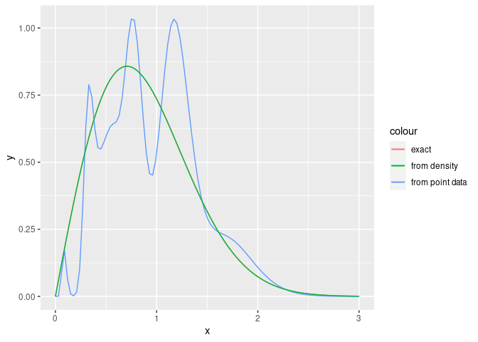
MAP (Markovian arrival process) is a stochastic point process whose
arrival rates are dominated by a CTMC. The CTMC expresses the internal
state of MAP called a phase process. MAP is generally defined by an
initial probability vector and two
matrices for infinitesimal generators
,
. Let
be the row
vector whose i-th entry is the probability that the phase process is i
at time t and n arrivals occur before time t. Then we have the following
differential equations:
[ \frac{d}{dt} \boldsymbol{\pi}(n,t) = \boldsymbol{\pi}(n,t) \boldsymbol{D}_0 + \boldsymbol{\pi}(n-1,t) \boldsymbol{D}_1, \quad \text{for \(n = 1, 2, \\ldots\)},](https://latex.codecogs.com/png.image?%5Cdpi%7B110%7D&space;%5Cbg_white&space;%0A%5Cfrac%7Bd%7D%7Bdt%7D%20%5Cboldsymbol%7B%5Cpi%7D%28n%2Ct%29%20%3D%20%5Cboldsymbol%7B%5Cpi%7D%28n%2Ct%29%20%5Cboldsymbol%7BD%7D_0%20%2B%20%5Cboldsymbol%7B%5Cpi%7D%28n-1%2Ct%29%20%5Cboldsymbol%7BD%7D_1%2C%20%5Cquad%20%5Ctext%7Bfor%20%24n%20%3D%201%2C%202%2C%20%5Cldots%24%7D%2C%0A ” (n,t) = (n,t) _0 + (n-1,t) _1, , “)
[ \frac{d}{dt} \boldsymbol{\pi}(0,t) = \boldsymbol{\pi}(0,t) \boldsymbol{D}_0, \quad \boldsymbol{\pi}(0,0) = \boldsymbol{\alpha},](https://latex.codecogs.com/png.image?%5Cdpi%7B110%7D&space;%5Cbg_white&space;%0A%5Cfrac%7Bd%7D%7Bdt%7D%20%5Cboldsymbol%7B%5Cpi%7D%280%2Ct%29%20%3D%20%5Cboldsymbol%7B%5Cpi%7D%280%2Ct%29%20%5Cboldsymbol%7BD%7D_0%2C%20%5Cquad%20%5Cboldsymbol%7B%5Cpi%7D%280%2C0%29%20%3D%20%5Cboldsymbol%7B%5Calpha%7D%2C%0A ” (0,t) = (0,t) _0, (0,0) = , “)
where and
are infinitesimal
generators of phase process without and with arrivals, respectively.
Note that
becomes the infinitesimal
generator of phase process. Similar to PH fitting, the purpose of MAP
fitting is to find MAP parameters
,
and
so that the estimated
MAP fits to observed data. In MAP fitting, there are also two
approaches; MM method and MLE. The MM method for MAP is to determine MAP
parameters with marginal/joint moments and k-lag correlation [1]. MLE is
to find MAP parameters maximizing the log-likelihood function. We
implement MLE approaches in the tool.
mapfit deals with point data and grouped data in MAP fitting. The point data for MAP fitting is a time series for arrivals. The grouped data for MAP fitting consists of break points and counts which are made from a time series for arrivals.
| Arrival No. | Time (sec) |
|---|---|
| 1 | 1.340 |
| 2 | 1.508 |
| 3 | 4.176 |
| 4 | 8.140 |
| 5 | 11.036 |
| 6 | 15.072 |
| 7 | 17.892 |
| 8 | 20.604 |
| 9 | 22.032 |
| 10 | 24.300 |
| … | … |
The above table shows an example of point data that consists of arrival times.
| Time interval | Counts |
|---|---|
| [0, 5] | 3 |
| [5, 10] | 1 |
| [10, 15] | 1 |
| [15, 20] | 2 |
| [20, 25] | 4 |
| … | … |
The above table shows an example of grouped data. The grouped data is made from the point data by counting the number of arrivals in every 5 seconds. Note that missing values cannot be treated in MAP fitting of this version of tool.
mapfit has three classes (models) for MAP, which have different parameter estimation algorithms.
map in the tool. Also, the tool uses a
Markov modulated Poisson process (MMPP) as a specific structure of
map, which can be generated by an mmpp
command.erhmm.gmmpp in the tool, and is
essentially same as mmpp except for parameter estimation
algorithm. In the parameter estimation of gmmpp, it is
assumed that at most one phase change is allowed in one observed time
interval [3].The map class consists of parameters ,
and
, which are given by slots of S4 class in R. The
gmmpp class also has the slots alpha,
D0 and D1 as model parameters. The
erhmm class has an initial probability vector for HMM
states (alpha), a probability transition matrix for HMM
states (P), the shape parameters for Erlang distribution
(shape) and the rate parameters for Erlang distribution
(rate). The S4 class erhmm can be transformed
to map by using as method.
The tool has the follwoing MAP fitting functions:
mapfit.point: MLEs for general MAP and ER-HMM from
point data. The estimation algorithm for general MAP is the EM algorithm
introduced in [4]. The algorithm for ER-HMM is the EM algorithm proposed
in [2].mapfit.group: MLEs for general MAP and
gmmpp from grouped data. Both the estimation algorithms for
general MAP and gmmpp are presented in [3]. Note that
erhmm cannot be used in the case of grouped data.The functions mapfit.point and mapfit.group
select an appropriate algorithm depending on the class of a given MAP.
These functions return a list including the estimated model
(map, erhmm or gmmpp), the
maximum log-likelihood (llf), Akaike information criterion (aic) and
other statistics of the estimation algorithm. In general,
erhmm for point data and gmmpp for grouped
data are much faster than general MAP.
Here we demonstrate MAP fitting with point and grouped data. The data used in this example is the traffic data; BCpAug89, which consists of time intervals for packet arrivals and is frequently used in several papers as a benchmark. We use only the first 1000 arrival times.
data(BCpAug89)
BCpAug89
#>    [1] 0.001340 0.000168 0.002668 0.003964 0.002896 0.004036 0.002820 0.002712
#>    [9] 0.001428 0.002268 0.000452 0.002604 0.001336 0.002148 0.000768 0.004236
#>   [17] 0.002624 0.004056 0.001520 0.001280 0.001972 0.001952 0.001112 0.001824
#>   [25] 0.001636 0.002536 0.002688 0.003984 0.002872 0.004132 0.002728 0.003968
#>   [33] 0.002888 0.004116 0.002744 0.004008 0.002848 0.004160 0.004340 0.003920
#>   [41] 0.004580 0.004008 0.004492 0.003920 0.002940 0.004080 0.002780 0.003960
#>   [49] 0.002896 0.001104 0.002836 0.000712 0.002208 0.000840 0.003172 0.000088
#>   [57] 0.002756 0.003932 0.002928 0.004128 0.002732 0.004056 0.002800 0.004016
#>   [65] 0.002844 0.003324 0.000620 0.002912 0.000956 0.003688 0.000360 0.003496
#>   [73] 0.001436 0.002592 0.002832 0.001280 0.002688 0.002892 0.001432 0.001956
#>   [81] 0.000576 0.001392 0.000888 0.001064 0.000144 0.001804 0.001956 0.000084
#>   [89] 0.000156 0.001612 0.001248 0.001652 0.001756 0.000552 0.002900 0.004000
#>   [97] 0.002856 0.003984 0.002876 0.004584 0.000164 0.001104 0.001528 0.001200
#>  [105] 0.000148 0.001096 0.001388 0.002188 0.000084 0.002716 0.001720 0.000148
#>  [113] 0.004716 0.003784 0.000084 0.003936 0.000204 0.002636 0.003956 0.012168
#>  [121] 0.001144 0.001472 0.001108 0.001304 0.001196 0.002184 0.002096 0.001108
#>  [129] 0.016220 0.003920 0.004060 0.003324 0.028744 0.003952 0.005580 0.003424
#>  [137] 0.003156 0.003388 0.015112 0.023060 0.002976 0.004532 0.012904 0.019180
#>  [145] 0.003112 0.004508 0.018756 0.000140 0.000768 0.003396 0.005956 0.012120
#>  [153] 0.004668 0.001752 0.016572 0.004792 0.015208 0.001152 0.008104 0.003320
#>  [161] 0.004512 0.043832 0.003076 0.005404 0.001288 0.001652 0.001076 0.008108
#>  [169] 0.002244 0.003576 0.030056 0.012236 0.003944 0.000164 0.000976 0.003416
#>  [177] 0.000980 0.001956 0.001964 0.000168 0.000140 0.001640 0.001956 0.000148
#>  [185] 0.001808 0.001636 0.000568 0.001912 0.000100 0.000832 0.000904 0.002944
#>  [193] 0.000224 0.002788 0.001120 0.003092 0.000584 0.002060 0.003944 0.002916
#>  [201] 0.000652 0.003264 0.002940 0.004384 0.004116 0.004064 0.002796 0.004192
#>  [209] 0.002668 0.003920 0.002936 0.004088 0.002768 0.001236 0.000840 0.001764
#>  [217] 0.000076 0.000352 0.002592 0.000532 0.003452 0.000608 0.002268 0.001268
#>  [225] 0.002700 0.002892 0.004120 0.000192 0.002544 0.003968 0.002888 0.003984
#>  [233] 0.002876 0.004200 0.004024 0.000276 0.000304 0.004832 0.005004 0.004228
#>  [241] 0.004272 0.000156 0.004052 0.002652 0.004060 0.000520 0.002280 0.003944
#>  [249] 0.002912 0.000084 0.004092 0.002684 0.004004 0.002852 0.004036 0.002824
#>  [257] 0.004392 0.000168 0.003940 0.000688 0.003492 0.002676 0.003936 0.002924
#>  [265] 0.004152 0.002704 0.003840 0.000312 0.002708 0.002640 0.001368 0.002852
#>  [273] 0.003956 0.002900 0.004164 0.002696 0.003968 0.000108 0.002780 0.000892
#>  [281] 0.003096 0.002872 0.003448 0.000576 0.002832 0.001240 0.002696 0.000236
#>  [289] 0.002688 0.001832 0.002312 0.002712 0.004308 0.002552 0.004028 0.002832
#>  [297] 0.003964 0.002200 0.000692 0.004308 0.002060 0.002132 0.000888 0.003136
#>  [305] 0.001380 0.001456 0.004020 0.002836 0.003976 0.002884 0.003960 0.002900
#>  [313] 0.003960 0.002896 0.002912 0.001132 0.002816 0.003996 0.001664 0.001196
#>  [321] 0.002340 0.000148 0.001464 0.002908 0.003924 0.002936 0.003972 0.002884
#>  [329] 0.004244 0.002616 0.003980 0.008076 0.004772 0.021240 0.001952 0.001960
#>  [337] 0.001952 0.001952 0.001952 0.001620 0.002560 0.001756 0.000712 0.003684
#>  [345] 0.002668 0.004584 0.007092 0.003952 0.010564 0.007516 0.019044 0.003540
#>  [353] 0.003044 0.003488 0.010200 0.003564 0.004072 0.003504 0.052540 0.003036
#>  [361] 0.005444 0.012124 0.037332 0.020336 0.004356 0.018748 0.003760 0.007084
#>  [369] 0.004576 0.014284 0.003084 0.004572 0.001260 0.000148 0.001328 0.001116
#>  [377] 0.001288 0.001284 0.002244 0.002076 0.001112 0.003028 0.005656 0.025340
#>  [385] 0.001140 0.001476 0.001188 0.001236 0.001264 0.002204 0.002012 0.001184
#>  [393] 0.006656 0.007248 0.003992 0.004512 0.004108 0.002748 0.004016 0.000164
#>  [401] 0.001244 0.001200 0.000236 0.001212 0.001156 0.001524 0.001312 0.000872
#>  [409] 0.002876 0.000148 0.001184 0.003788 0.003528 0.002928 0.001020 0.000120
#>  [417] 0.002788 0.004024 0.000168 0.001788 0.000880 0.001080 0.001952 0.001180
#>  [425] 0.000896 0.001828 0.000148 0.002688 0.001940 0.000888 0.000888 0.000892
#>  [433] 0.000168 0.000888 0.001428 0.000360 0.000948 0.001396 0.002340 0.000076
#>  [441] 0.002948 0.000792 0.001376 0.001300 0.001400 0.000164 0.000996 0.001540
#>  [449] 0.001132 0.001208 0.000148 0.002032 0.002796 0.000168 0.001308 0.000084
#>  [457] 0.002112 0.004188 0.000172 0.002500 0.003972 0.002884 0.002368 0.001620
#>  [465] 0.002868 0.003988 0.002872 0.003960 0.003632 0.000144 0.001164 0.001296
#>  [473] 0.001240 0.001268 0.000168 0.001312 0.002052 0.000176 0.003188 0.001508
#>  [481] 0.000164 0.002860 0.001112 0.000144 0.001056 0.001196 0.001212 0.001196
#>  [489] 0.000284 0.001916 0.001940 0.000144 0.000980 0.000148 0.000080 0.003504
#>  [497] 0.001704 0.000952 0.001132 0.002648 0.001644 0.001860 0.000708 0.004068
#>  [505] 0.002788 0.003940 0.001256 0.001424 0.000240 0.000972 0.001404 0.002040
#>  [513] 0.001764 0.000168 0.002808 0.000080 0.001132 0.000148 0.001508 0.001192
#>  [521] 0.001328 0.001260 0.000168 0.001292 0.001116 0.000084 0.000552 0.000540
#>  [529] 0.001204 0.001744 0.001552 0.003308 0.000212 0.003988 0.002868 0.004108
#>  [537] 0.002752 0.003952 0.002904 0.004148 0.001212 0.000084 0.001212 0.000204
#>  [545] 0.001592 0.001112 0.001256 0.001268 0.000168 0.002016 0.001088 0.000888
#>  [553] 0.001228 0.003940 0.002444 0.003960 0.002896 0.002528 0.001716 0.002616
#>  [561] 0.001488 0.002480 0.000476 0.002264 0.000152 0.003332 0.000620 0.002904
#>  [569] 0.004868 0.000160 0.001068 0.001228 0.001224 0.000144 0.001064 0.001224
#>  [577] 0.001428 0.000304 0.002680 0.000160 0.001056 0.003172 0.002632 0.004044
#>  [585] 0.002812 0.002268 0.001768 0.002224 0.001236 0.000144 0.003956 0.002900
#>  [593] 0.004052 0.002812 0.004004 0.001652 0.001200 0.001328 0.002132 0.000548
#>  [601] 0.001812 0.000076 0.000964 0.003972 0.001724 0.001160 0.000980 0.002972
#>  [609] 0.000172 0.001200 0.001352 0.000184 0.002036 0.001480 0.000556 0.002224
#>  [617] 0.000560 0.003060 0.001416 0.000132 0.000168 0.000892 0.001428 0.001104
#>  [625] 0.000172 0.000148 0.000960 0.002184 0.000916 0.001028 0.000168 0.000996
#>  [633] 0.000144 0.002104 0.002320 0.002976 0.001324 0.001880 0.003972 0.002888
#>  [641] 0.003976 0.004524 0.004012 0.002844 0.000988 0.001132 0.001468 0.001112
#>  [649] 0.000168 0.001040 0.001488 0.001308 0.001180 0.002056 0.001124 0.004504
#>  [657] 0.005872 0.001156 0.005652 0.020652 0.001220 0.001476 0.001316 0.000888
#>  [665] 0.000912 0.000888 0.000904 0.000888 0.000900 0.000920 0.000888 0.000908
#>  [673] 0.000888 0.000080 0.000140 0.000956 0.000924 0.001104 0.000904 0.000888
#>  [681] 0.000900 0.000892 0.001116 0.001172 0.001952 0.001120 0.004940 0.004420
#>  [689] 0.005244 0.002152 0.002756 0.000132 0.002144 0.001800 0.003008 0.003120
#>  [697] 0.001116 0.001264 0.001360 0.000888 0.001068 0.000136 0.000892 0.000932
#>  [705] 0.000380 0.001572 0.000888 0.001068 0.000132 0.001400 0.000892 0.000372
#>  [713] 0.000924 0.002772 0.000432 0.001328 0.000888 0.000888 0.000892 0.000296
#>  [721] 0.000892 0.001704 0.001108 0.001296 0.001252 0.000216 0.001284 0.001604
#>  [729] 0.000600 0.002020 0.001204 0.000304 0.007224 0.011096 0.002204 0.002172
#>  [737] 0.004148 0.004224 0.006592 0.004080 0.004132 0.004592 0.005516 0.002524
#>  [745] 0.001428 0.003048 0.001820 0.002316 0.001596 0.001496 0.001564 0.002492
#>  [753] 0.002924 0.000372 0.002024 0.003456 0.004376 0.002008 0.002512 0.004336
#>  [761] 0.005000 0.003040 0.001152 0.002804 0.000860 0.002180 0.000928 0.002440
#>  [769] 0.001152 0.004024 0.003624 0.000372 0.002156 0.003704 0.003004 0.003484
#>  [777] 0.002828 0.003572 0.004444 0.004920 0.000140 0.001072 0.004016 0.003604
#>  [785] 0.003876 0.003832 0.002500 0.003608 0.004088 0.006196 0.014896 0.005340
#>  [793] 0.000132 0.004648 0.001136 0.003416 0.003116 0.004452 0.000088 0.002456
#>  [801] 0.002252 0.006692 0.001156 0.002248 0.001324 0.001816 0.002540 0.000656
#>  [809] 0.004140 0.000320 0.003344 0.000612 0.002764 0.002160 0.000224 0.004192
#>  [817] 0.002836 0.003076 0.002732 0.000488 0.004060 0.000988 0.003452 0.004052
#>  [825] 0.002808 0.004108 0.001308 0.001440 0.004068 0.002792 0.004212 0.002648
#>  [833] 0.004120 0.002736 0.003956 0.001048 0.001856 0.002048 0.002156 0.001328
#>  [841] 0.001324 0.000888 0.003200 0.000168 0.002604 0.002240 0.001544 0.000336
#>  [849] 0.001800 0.000940 0.000452 0.002616 0.000452 0.002444 0.000240 0.000732
#>  [857] 0.002888 0.000316 0.004088 0.000168 0.002600 0.000536 0.002716 0.000324
#>  [865] 0.000596 0.002688 0.000100 0.000084 0.003372 0.000736 0.000276 0.002212
#>  [873] 0.001720 0.000592 0.001692 0.002500 0.000272 0.001492 0.001952 0.001084
#>  [881] 0.000404 0.003276 0.000984 0.002008 0.000168 0.000576 0.001204 0.001956
#>  [889] 0.000148 0.000128 0.000692 0.000980 0.001952 0.000144 0.001808 0.000084
#>  [897] 0.001560 0.001012 0.001544 0.000136 0.001628 0.000728 0.000784 0.003112
#>  [905] 0.000552 0.004052 0.000388 0.003788 0.000788 0.000188 0.001708 0.003984
#>  [913] 0.002872 0.004224 0.002636 0.003224 0.000824 0.002808 0.000148 0.003056
#>  [921] 0.000724 0.002676 0.000256 0.004148 0.002708 0.004000 0.001388 0.001472
#>  [929] 0.003476 0.003732 0.001148 0.000096 0.001148 0.001216 0.000216 0.001000
#>  [937] 0.001180 0.000140 0.000412 0.000556 0.000776 0.002336 0.000144 0.001008
#>  [945] 0.000096 0.001604 0.001416 0.001220 0.001516 0.003704 0.000572 0.002584
#>  [953] 0.001112 0.002820 0.000160 0.002764 0.004156 0.002704 0.003916 0.002944
#>  [961] 0.000784 0.003200 0.000244 0.003060 0.001208 0.002348 0.001572 0.002940
#>  [969] 0.004084 0.004168 0.000248 0.003336 0.000612 0.003756 0.000796 0.004172
#>  [977] 0.000100 0.000168 0.002956 0.001104 0.000160 0.001844 0.002764 0.000332
#>  [985] 0.001648 0.001752 0.000876 0.001800 0.001080 0.000288 0.001088 0.000912
#>  [993] 0.000812 0.001740 0.000236 0.000344 0.001860 0.002680 0.000900 0.000152
Using this point data, we can estimate parameters for general MAP with 5 states, MMPP with 5 states and ER-HMM with 5 states by the following commands, respectively;
## mapfit for general MAP
mapfit.point(map=map(5), x=cumsum(BCpAug89))
#>
#> Maximum LLF: 5140.147595
#> AIC: -10190.295190
#> Iteration:  1011 / 2000
#> Computation time (user): 13.964000
#> Convergence: TRUE
#> Error (abs): 7.646365e-05 (tolerance Inf)
#> Error (rel): 1.487577e-08 (tolerance 1.490116e-08)
#>
#> Size : 5
#> Initial :  0.1801396 0.2885964 0.1771319 0.1812461 0.172886
#> Infinitesimal generator :
#> 5 x 5 sparse Matrix of class "dgCMatrix"
#>
#> [1,] -1.061324e+03  5.235987e-02  1.127125e-25  9.839023e+02  2.183896e-04
#> [2,]  1.209889e-02 -1.123448e+02  1.188700e-01  1.291279e-02  2.573930e+00
#> [3,]  1.467385e-84  1.677555e+00 -1.074471e+03  4.891540e-36  1.396510e-48
#> [4,]  2.613107e-32  1.451876e+01  9.714023e+02 -1.021438e+03  2.750421e-12
#> [5,]  3.463362e-53  4.562652e-66  1.478035e-04  3.357871e-19 -8.272394e+02
#> 5 x 5 sparse Matrix of class "dgCMatrix"
#>
#> [1,] 7.688721e+01 3.729835e-211 2.281306e-122 1.229387e-36 4.823690e-01
#> [2,] 4.074875e+00  1.019899e+02  1.572422e+00 1.985961e+00 3.894666e-03
#> [3,] 9.944944e+02  2.842794e-01  7.775000e+01 6.219898e-22 2.646421e-01
#> [4,] 2.624369e-21  9.856690e-81  7.323236e-54 2.980665e-43 3.551686e+01
#> [5,] 5.989362e-09  3.343306e-76  1.008148e-10 4.231130e+01 7.849279e+02

## mapfit for general MMPP
mapfit.point(map=mmpp(5), x=cumsum(BCpAug89))
#>
#> Maximum LLF: 5055.133942
#> AIC: -10060.267883
#> Iteration:  404 / 2000
#> Computation time (user): 8.724000
#> Convergence: TRUE
#> Error (abs): 7.264097e-05 (tolerance Inf)
#> Error (rel): 1.436974e-08 (tolerance 1.490116e-08)
#>
#> Size : 5
#> Initial :  0.02144093 0.238745 0.401778 0.002786422 0.3352496
#> Infinitesimal generator :
#> 5 x 5 sparse Matrix of class "dgCMatrix"
#>
#> [1,] -844.276406  4.865555e-05  143.22925542    42.587977  181.9538205
#> [2,]    2.104589 -1.121355e+02    0.03553884     1.121266    1.5590542
#> [3,]    1.370654  2.864409e+00 -362.16740393     6.336612    0.1688801
#> [4,] 1880.457155  7.690769e-05  369.80585855 -2708.771347    5.1918483
#> [5,]    4.750041  1.419096e-15    0.61276819     7.629885 -653.0968904
#> 5 x 5 sparse Matrix of class "dgCMatrix"
#>
#> [1,] 476.5053   .       .        .        .
#> [2,]   .      107.315   .        .        .
#> [3,]   .        .     351.4268   .        .
#> [4,]   .        .       .      453.3164   .
#> [5,]   .        .       .        .      640.1042

## mapfit for ER-HMM
mapfit.point(map=erhmm(5), x=cumsum(BCpAug89))
#> shape:  1 1 1 1 1  llf=5055.11
#> shape:  1 1 1 2  llf=5113.70
#> shape:  1 1 3  llf=5121.86
#> shape:  1 2 2  llf=5106.48
#> shape:  1 4  llf=5003.21
#> shape:  2 3  llf=5024.03
#> shape:  5  llf=3716.53
#>
#> Maximum LLF: 5121.860147
#> AIC: -10221.720294
#> Iteration:  71 / 2000
#> Computation time (user): 1.260000
#> Convergence: TRUE
#> Error (abs): 6.302517e-05 (tolerance Inf)
#> Error (rel): 1.230513e-08 (tolerance 1.490116e-08)
#>
#> Size : 3
#> Shape   :  1 1 3
#> Initial :  0.4956884 0.08702657 0.417285
#> Rate    :  748.6684 111.8898 1061.68
#> Transition probability :
#> 3 x 3 sparse Matrix of class "dgCMatrix"
#>
#> [1,] 0.91943990 2.080601e-11 0.08056010
#> [2,] 0.03562065 9.053646e-01 0.05901477
#> [3,] 0.08826764 1.973662e-02 0.89199574
In the above example, cumsum is a function to derive
cumulative sums because BCpAug89 provides time difference
data. The estimation with erhmm is much faster than
others.
Next we present MAP fitting with grouped data. The grouped data is
made from BCpAug89 by using hist function,
i.e.,
BCpAug89.group<-hist(cumsum(BCpAug89), breaks=seq(0,2.7,0.01), plot=FALSE)

BCpAug89.group$breaks
#>   [1] 0.00 0.01 0.02 0.03 0.04 0.05 0.06 0.07 0.08 0.09 0.10 0.11 0.12 0.13 0.14
#>  [16] 0.15 0.16 0.17 0.18 0.19 0.20 0.21 0.22 0.23 0.24 0.25 0.26 0.27 0.28 0.29
#>  [31] 0.30 0.31 0.32 0.33 0.34 0.35 0.36 0.37 0.38 0.39 0.40 0.41 0.42 0.43 0.44
#>  [46] 0.45 0.46 0.47 0.48 0.49 0.50 0.51 0.52 0.53 0.54 0.55 0.56 0.57 0.58 0.59
#>  [61] 0.60 0.61 0.62 0.63 0.64 0.65 0.66 0.67 0.68 0.69 0.70 0.71 0.72 0.73 0.74
#>  [76] 0.75 0.76 0.77 0.78 0.79 0.80 0.81 0.82 0.83 0.84 0.85 0.86 0.87 0.88 0.89
#>  [91] 0.90 0.91 0.92 0.93 0.94 0.95 0.96 0.97 0.98 0.99 1.00 1.01 1.02 1.03 1.04
#> [106] 1.05 1.06 1.07 1.08 1.09 1.10 1.11 1.12 1.13 1.14 1.15 1.16 1.17 1.18 1.19
#> [121] 1.20 1.21 1.22 1.23 1.24 1.25 1.26 1.27 1.28 1.29 1.30 1.31 1.32 1.33 1.34
#> [136] 1.35 1.36 1.37 1.38 1.39 1.40 1.41 1.42 1.43 1.44 1.45 1.46 1.47 1.48 1.49
#> [151] 1.50 1.51 1.52 1.53 1.54 1.55 1.56 1.57 1.58 1.59 1.60 1.61 1.62 1.63 1.64
#> [166] 1.65 1.66 1.67 1.68 1.69 1.70 1.71 1.72 1.73 1.74 1.75 1.76 1.77 1.78 1.79
#> [181] 1.80 1.81 1.82 1.83 1.84 1.85 1.86 1.87 1.88 1.89 1.90 1.91 1.92 1.93 1.94
#> [196] 1.95 1.96 1.97 1.98 1.99 2.00 2.01 2.02 2.03 2.04 2.05 2.06 2.07 2.08 2.09
#> [211] 2.10 2.11 2.12 2.13 2.14 2.15 2.16 2.17 2.18 2.19 2.20 2.21 2.22 2.23 2.24
#> [226] 2.25 2.26 2.27 2.28 2.29 2.30 2.31 2.32 2.33 2.34 2.35 2.36 2.37 2.38 2.39
#> [241] 2.40 2.41 2.42 2.43 2.44 2.45 2.46 2.47 2.48 2.49 2.50 2.51 2.52 2.53 2.54
#> [256] 2.55 2.56 2.57 2.58 2.59 2.60 2.61 2.62 2.63 2.64 2.65 2.66 2.67 2.68 2.69
#> [271] 2.70

BCpAug89.group$counts
#>   [1]  4  3  6  4  5  5  2  4  2  3  2  3  3  3  5  5  2  3  5  5  4  8  8  3  4
#>  [26]  8  4  5  1  5  4  0  3  1  0  0  2  3  1  1  0  1  2  0  1  1  2  0  4  1
#>  [51]  1  2  0  2  0  2  3  0  0  0  0  2  4  3  0  0  1  0  5  9  8  5  4  2  3
#>  [76]  3  4  8  4  4  3  4  2  3  4  4  3  3  4  4  2  5  3  4  4  6  4  3  4  4
#> [101]  4  3  3  4  6  3  2  3  2  0  0  5  5  3  2  0  2  0  1  3  1  3  0  0  0
#> [126]  0  0  3  0  1  0  0  1  0  1  1  0  2  2  0  3  7  4  0  0  4  5  1  3  2
#> [151] 10  4  5  8  9  7 10  6  4  4  3  8  6 10  7  5  6  8 11  4  4  2 10  5  3
#> [176]  6  5  8  6  4  5  3  6  6  8  8 11  5  3  2  9  4  2  1  0  8 13  6  2  5
#> [201]  5 12 10  9  3  1  4  1  3  2  5  5  3  4  3  6  4  3  3  4  2  3  2  0  3
#> [226]  3  5  3  4  7  3  4  3  4  3  3  6  5  9  5  8  7  8 11  9  4  5  3  6  4
#> [251]  4 12  8  5  4  3  6  2  6  7  8  8  2  0  0  0  0  0  0  0
In the above, break points are set as a time point sequence from 0 to
2.7 by 0.01, which is generated by a seq function. Using
the grouped data, we have the estimated parameters for general MAP, MMPP
and MMPP with approximate estimation (gmmpp).
## mapfit for general MAP with grouped data
mapfit.group(map=map(5), counts=BCpAug89.group$counts, breaks=BCpAug89.group$breaks)
#>
#> Maximum LLF: -543.092984
#> AIC: 1176.185967
#> Iteration:  1384 / 2000
#> Computation time (user): 51.224000
#> Convergence: TRUE
#> Error (abs): 8.082774e-06 (tolerance Inf)
#> Error (rel): 1.488285e-08 (tolerance 1.490116e-08)
#>
#> Size : 5
#> Initial :  0.07333445 0.2487455 0.1723761 0.322209 0.1833349
#> Infinitesimal generator :
#> 5 x 5 sparse Matrix of class "dgCMatrix"
#>
#> [1,]  -3.047904e+01  3.947300e-159   1.422234e-30  1.592732e-90   6.332886e-32
#> [2,]  5.494354e-211  -1.102898e+02  5.692130e-320  1.461261e-17  1.219775e-315
#> [3,]   2.348635e-13   3.359617e-02  -7.633223e+02  8.883249e+00   2.059710e-05
#> [4,]   1.508458e-01   1.453163e+00   9.181767e-03 -6.389108e+02   5.970120e-04
#> [5,]   3.718644e-13   2.536356e-02   6.999167e+02  2.030370e-03  -7.055768e+02
#> 5 x 5 sparse Matrix of class "dgCMatrix"
#>
#> [1,] 4.046247e-293 1.724406e-115  3.047904e+01 8.542693e-87  6.102553e-29
#> [2,] 8.445178e-279  1.050356e+02 3.123209e-310 5.254179e+00 6.617169e-319
#> [3,]  1.956194e-10  4.377445e+00  7.441963e-03 2.244253e-04  7.500203e+02
#> [4,]  3.752686e+00  5.794493e-02  3.165501e+00 6.301008e+02  2.200785e-01
#> [5,]  5.331282e+00  3.002839e-01  2.479617e-08 2.000958e-04  9.440298e-04

## mapfit for general MMPP with grouped data
mapfit.group(map=mmpp(5), counts=BCpAug89.group$counts, breaks=BCpAug89.group$breaks)
#> Warning in emfit(map, data, initialize = FALSE, ufact = con$uniform.factor, :
#> LLF decreses: iter=132 llf.diff=4.220933e-05
#> Warning in emfit(map, data, initialize = FALSE, ufact = con$uniform.factor, :
#> LLF decreses: iter=133 llf.diff=3.366376e-04
#> Warning in emfit(map, data, initialize = FALSE, ufact = con$uniform.factor, :
#> LLF decreses: iter=134 llf.diff=5.051768e-04
#> Warning in emfit(map, data, initialize = FALSE, ufact = con$uniform.factor, :
#> LLF decreses: iter=135 llf.diff=5.845536e-04
#> Warning in emfit(map, data, initialize = FALSE, ufact = con$uniform.factor, :
#> LLF decreses: iter=136 llf.diff=6.038050e-04
#> Warning in emfit(map, data, initialize = FALSE, ufact = con$uniform.factor, :
#> LLF decreses: iter=137 llf.diff=5.848563e-04
#> Warning in emfit(map, data, initialize = FALSE, ufact = con$uniform.factor, :
#> LLF decreses: iter=138 llf.diff=5.435768e-04
#> Warning in emfit(map, data, initialize = FALSE, ufact = con$uniform.factor, :
#> LLF decreses: iter=139 llf.diff=4.909857e-04
#> Warning in emfit(map, data, initialize = FALSE, ufact = con$uniform.factor, :
#> LLF decreses: iter=140 llf.diff=4.344059e-04
#> Warning in emfit(map, data, initialize = FALSE, ufact = con$uniform.factor, :
#> LLF decreses: iter=141 llf.diff=3.784562e-04
#> Warning in emfit(map, data, initialize = FALSE, ufact = con$uniform.factor, :
#> LLF decreses: iter=142 llf.diff=3.258503e-04
#> Warning in emfit(map, data, initialize = FALSE, ufact = con$uniform.factor, :
#> LLF decreses: iter=143 llf.diff=2.780067e-04
#> Warning in emfit(map, data, initialize = FALSE, ufact = con$uniform.factor, :
#> LLF decreses: iter=144 llf.diff=2.354965e-04
#> Warning in emfit(map, data, initialize = FALSE, ufact = con$uniform.factor, :
#> LLF decreses: iter=145 llf.diff=1.983613e-04
#> Warning in emfit(map, data, initialize = FALSE, ufact = con$uniform.factor, :
#> LLF decreses: iter=146 llf.diff=1.663313e-04
#> Warning in emfit(map, data, initialize = FALSE, ufact = con$uniform.factor, :
#> LLF decreses: iter=147 llf.diff=1.389718e-04
#> Warning in emfit(map, data, initialize = FALSE, ufact = con$uniform.factor, :
#> LLF decreses: iter=148 llf.diff=1.157771e-04
#> Warning in emfit(map, data, initialize = FALSE, ufact = con$uniform.factor, :
#> LLF decreses: iter=149 llf.diff=9.622870e-05
#> Warning in emfit(map, data, initialize = FALSE, ufact = con$uniform.factor, :
#> LLF decreses: iter=150 llf.diff=7.983006e-05
#> Warning in emfit(map, data, initialize = FALSE, ufact = con$uniform.factor, :
#> LLF decreses: iter=151 llf.diff=6.612451e-05
#> Warning in emfit(map, data, initialize = FALSE, ufact = con$uniform.factor, :
#> LLF decreses: iter=152 llf.diff=5.470362e-05
#> Warning in emfit(map, data, initialize = FALSE, ufact = con$uniform.factor, :
#> LLF decreses: iter=153 llf.diff=4.520912e-05
#> Warning in emfit(map, data, initialize = FALSE, ufact = con$uniform.factor, :
#> LLF decreses: iter=154 llf.diff=3.733118e-05
#> Warning in emfit(map, data, initialize = FALSE, ufact = con$uniform.factor, :
#> LLF decreses: iter=155 llf.diff=3.080462e-05
#> Warning in emfit(map, data, initialize = FALSE, ufact = con$uniform.factor, :
#> LLF decreses: iter=156 llf.diff=2.540439e-05
#> Warning in emfit(map, data, initialize = FALSE, ufact = con$uniform.factor, :
#> LLF decreses: iter=157 llf.diff=2.094063e-05
#> Warning in emfit(map, data, initialize = FALSE, ufact = con$uniform.factor, :
#> LLF decreses: iter=158 llf.diff=1.725397e-05
#> Warning in emfit(map, data, initialize = FALSE, ufact = con$uniform.factor, :
#> LLF decreses: iter=159 llf.diff=1.421116e-05
#> Warning in emfit(map, data, initialize = FALSE, ufact = con$uniform.factor, :
#> LLF decreses: iter=160 llf.diff=1.170111e-05
#> Warning in emfit(map, data, initialize = FALSE, ufact = con$uniform.factor, :
#> LLF decreses: iter=161 llf.diff=9.631476e-06
#> Warning in emfit(map, data, initialize = FALSE, ufact = con$uniform.factor, :
#> LLF decreses: iter=162 llf.diff=7.925587e-06
#>
#> Maximum LLF: -558.890363
#> AIC: 1167.780726
#> Iteration:  162 / 2000
#> Computation time (user): 5.392000
#> Convergence: TRUE
#> Error (abs): 7.925587e-06 (tolerance Inf)
#> Error (rel): 1.418093e-08 (tolerance 1.490116e-08)
#>
#> Size : 5
#> Initial :  0.336854 0.1773842 0.3521996 0.1275778 0.005984325
#> Infinitesimal generator :
#> 5 x 5 sparse Matrix of class "dgCMatrix"
#>
#> [1,] -99.872163  4.580554e-07    7.248944  7.308010e-07  5.354417e-07
#> [2,]   1.524902 -4.724140e+02    2.329234  9.475050e+01  1.416705e+01
#> [3,]   5.248968  2.461266e+00 -631.368618  1.141778e+00  4.811211e-01
#> [4,]   2.299920  1.491683e+02    2.076641 -5.287208e+02  1.580929e+01
#> [5,]   4.886126  1.779647e+01   27.937475  7.346608e+02 -1.144126e+03
#> 5 x 5 sparse Matrix of class "dgCMatrix"
#>
#> [1,] 92.62322   .        .        .        .
#> [2,]  .       359.6423   .        .        .
#> [3,]  .         .      622.0355   .        .
#> [4,]  .         .        .      359.3667   .
#> [5,]  .         .        .        .      358.8456

## mapfit for general MMPP with grouped data (approximation)
mapfit.group(map=gmmpp(5), counts=BCpAug89.group$counts, breaks=BCpAug89.group$breaks)
#>
#> Maximum LLF: -828.051682
#> AIC: 1706.103365
#> Iteration:  102 / 2000
#> Computation time (user): 2.943000
#> Convergence: TRUE
#> Error (abs): 1.213698e-05 (tolerance Inf)
#> Error (rel): 1.465727e-08 (tolerance 1.490116e-08)
#>
#> Size : 5
#> Initial :  0.07402404 0.2640609 0.3241613 0.1628244 0.1749294
#> Infinitesimal generator :
#> 5 x 5 Matrix of class "dgeMatrix"
#>               [,1]          [,2]          [,3]          [,4]          [,5]
#> [1,] -1.090465e+03  1.460739e-05   95.43625590  1.975754e-14  8.219658e-09
#> [2,]  1.744402e-05 -4.659664e+02   90.09109238  2.693177e-08  9.094447e+00
#> [3,]  1.931501e+01  8.079529e+01 -571.48907351  5.930851e-09  7.751839e-08
#> [4,]  2.794275e-14  1.946525e-03    0.01169835 -9.466821e+01  9.465456e+01
#> [5,]  4.592685e+00  5.077813e-06    9.12293102  8.811722e+01 -2.984222e+02
#> 5 x 5 Matrix of class "dgeMatrix"
#>          [,1]     [,2]     [,3]         [,4]     [,5]
#> [1,] 995.0287   0.0000   0.0000 0.000000e+00   0.0000
#> [2,]   0.0000 366.7809   0.0000 0.000000e+00   0.0000
#> [3,]   0.0000   0.0000 471.3788 0.000000e+00   0.0000
#> [4,]   0.0000   0.0000   0.0000 1.022278e-06   0.0000
#> [5,]   0.0000   0.0000   0.0000 0.000000e+00 196.5894