mixgb

mixgb is a scalable multiple imputation framework based on XGBoost, bootstrapping and predictive mean matching. The proposed framework is implemented in an R package mixgb. We have shown that our framework obtains less biased estimates and reflects appropriate imputation variability, while achieving high computational efficiency. For more details, please check our paper https://arxiv.org/abs/2106.01574. (Our package has been revised and updated since the preprint was posted. Simulation code in the original supplementary files may not run as expected. Revised paper and adapted code will be updated soon.)

New updates

May 2022

• Visual diagnostic functions of multiply imputed data
• Use S3 instead of R6
• Plot functions can show masked missing data (if provided)

April 2022

• User can now set different number of iterations maxit.
• Both single and multiple imputation with XGBoost can do predictive mean matching
• Bootstrap data to make m imputations is optional. User can set bootstrap = FALSE to disable bootstrap. Users can also set sampling related hyperparameters of XGBoost (subsample, colsample_bytree, colsample_bylevel, colsample_bynode) to be less than 1 to achieve similar effect.
• Add predicted mean matching type 0. Now the options for pmm.type are NULL,0,1,2 or "auto" (type 2 for numeric/integer variables, no PMM for categorical variables).
• Added more validation checks
• Compatible with data.table
• Cross-validation to pre-tune nrounds

Under development

• make m imputation parallel
• pre-tune other hyperparameters

Notice

• Currently users can set XGBoost parameter nthread for multithreading with OpenMP support. However, MacOS has disabled OpenMP support.

1. Installation

You can install the development version of mixgb from GitHub with:

# install.packages("devtools")
devtools::install_github("agnesdeng/mixgb")

# load mixgb
library(mixgb)

1.1 Data cleaning before imputation

It is highly recommended to clean and check your data before imputation. Here are some common issues:

• Data should be a data frame.
• ID should be removed
• Missing values should be coded as NA not NaN
• Inf or -Inf are not allowed
• Empty cells should be coded as NA or sensible values
• Variables of “character” type should be converted to “factor” instead
• Variables of “factor” type should have at least two levels

The function data_clean() can do a preliminary check and fix some obvious problems. However, it would not fix all issues related to data quality.

cleanWithNA.df <- data_clean(rawdata)

2. Impute missing values with mixgb

We first load the mixgb package and the nhanes3_newborn dataset, which contains 16 variables of various types (integer/numeric/factor/ordinal factor). There are 9 variables with missing values.

str(nhanes3_newborn)
#> tibble [2,107 × 16] (S3: tbl_df/tbl/data.frame)
#>  $ HSHSIZER: int [1:2107] 4 3 5 4 4 3 5 3 3 3 ...
#>  $ HSAGEIR : int [1:2107] 2 5 10 10 8 3 10 7 2 7 ...
#>  $ HSSEX   : Factor w/ 2 levels "1","2": 2 1 2 2 1 1 2 2 2 1 ...
#>  $ DMARACER: Factor w/ 3 levels "1","2","3": 1 1 2 1 1 1 2 1 2 2 ...
#>  $ DMAETHNR: Factor w/ 3 levels "1","2","3": 3 1 3 3 3 3 3 3 3 3 ...
#>  $ DMARETHN: Factor w/ 4 levels "1","2","3","4": 1 3 2 1 1 1 2 1 2 2 ...
#>  $ BMPHEAD : num [1:2107] 39.3 45.4 43.9 45.8 44.9 42.2 45.8 NA 40.2 44.5 ...
#>   ..- attr(*, "label")= chr "Head circumference (cm)"
#>  $ BMPRECUM: num [1:2107] 59.5 69.2 69.8 73.8 69 61.7 74.8 NA 64.5 70.2 ...
#>   ..- attr(*, "label")= chr "Recumbent length (cm)"
#>  $ BMPSB1  : num [1:2107] 8.2 13 6 8 8.2 9.4 5.2 NA 7 5.9 ...
#>   ..- attr(*, "label")= chr "First subscapular skinfold (mm)"
#>  $ BMPSB2  : num [1:2107] 8 13 5.6 10 7.8 8.4 5.2 NA 7 5.4 ...
#>   ..- attr(*, "label")= chr "Second subscapular skinfold (mm)"
#>  $ BMPTR1  : num [1:2107] 9 15.6 7 16.4 9.8 9.6 5.8 NA 11 6.8 ...
#>   ..- attr(*, "label")= chr "First triceps skinfold (mm)"
#>  $ BMPTR2  : num [1:2107] 9.4 14 8.2 12 8.8 8.2 6.6 NA 10.9 7.6 ...
#>   ..- attr(*, "label")= chr "Second triceps skinfold (mm)"
#>  $ BMPWT   : num [1:2107] 6.35 9.45 7.15 10.7 9.35 7.15 8.35 NA 7.35 8.65 ...
#>   ..- attr(*, "label")= chr "Weight (kg)"
#>  $ DMPPIR  : num [1:2107] 3.186 1.269 0.416 2.063 1.464 ...
#>   ..- attr(*, "label")= chr "Poverty income ratio"
#>  $ HFF1    : Factor w/ 2 levels "1","2": 2 2 1 1 1 2 2 1 2 1 ...
#>  $ HYD1    : Ord.factor w/ 5 levels "1"<"2"<"3"<"4"<..: 1 3 1 1 1 1 1 1 2 1 ...
colSums(is.na(nhanes3_newborn))
#> HSHSIZER  HSAGEIR    HSSEX DMARACER DMAETHNR DMARETHN  BMPHEAD BMPRECUM 
#>        0        0        0        0        0        0      124      114 
#>   BMPSB1   BMPSB2   BMPTR1   BMPTR2    BMPWT   DMPPIR     HFF1     HYD1 
#>      161      169      124      167      117      192        7        0

To impute this dataset, we can use the default settings. The default number of imputed datasets m = 5. Note that we do not need to convert our data into dgCMatrix or one-hot coding format. Our package will convert it automatically. Variables should be of the following types: numeric, integer, factor or ordinal factor.

# use mixgb with default settings
imputed.data <- mixgb(data = nhanes3_newborn, m = 5)

2.1 Customise imputation settings

We can also customise imputation settings:

• The number of imputed datasets m

• The number of imputation iterations maxit

• Whether to convert ordinal factors to integer (imputation process will be faster) ordinalAsInteger

• Whether to use bootstrapping bootstrap

• Predictive mean matching settings pmm.type, pmm.k and pmm.link.

• Initial imputation methods for different types of variables initial.num, initial.int and initial.fac.

• Whether to save models for imputing newdata save.models and save.vars.

• XGBoost hyperparameters and verbose settings. xgb.params, nrounds, early_stopping_rounds, print_every_n and verbose.

# Use mixgb with chosen settings
params <- list(max_depth = 6, gamma = 0.1, eta = 0.3, min_child_weight = 1,
    subsample = 1, colsample_bytree = 1, colsample_bylevel = 1,
    colsample_bynode = 1, nthread = 4, tree_method = "auto",
    gpu_id = 0, predictor = "auto")

imputed.data <- mixgb(data = nhanes3_newborn, m = 5, maxit = 1,
    ordinalAsInteger = TRUE, bootstrap = TRUE, pmm.type = "auto",
    pmm.k = 5, pmm.link = "prob", initial.num = "normal", initial.int = "mode",
    initial.fac = "mode", save.models = FALSE, save.vars = NULL,
    xgb.params = params, nrounds = 50, early_stopping_rounds = 10,
    print_every_n = 10L, verbose = 0)

2.2 Tune hyperparameters

Imputation performance can be affected by the hyperparameter settings. It may seem daunting to tune a large set of hyperparameters, but often we can narrow down the search as many hyperparameters are correlated. In our package, we have a function mixgb_cv() to tune nrounds. There is no default nrounds value in XGBoost, so we need to specify it. The default nrounds in mixgb is 50. However, we recommend using mixgb_cv() to find the optimal nrounds first.

cv.results <- mixgb_cv(data = nhanes3_newborn, verbose = FALSE)
cv.results$response
#> [1] "BMPWT"
cv.results$best.nrounds
#> [1] 18

By default, mixgb_cv() will randomly choose an incomplete variable as the response and build an XGBoost model with other variables using the complete cases of the dataset. Therefore, each run of mixgb_cv() is likely to return different results. Users can also specify the response and covariates in the argument response and select_features, respectively.

cv.results <- mixgb_cv(data = nhanes3_newborn, nfold = 10, nrounds = 100,
    early_stopping_rounds = 1, response = "BMPHEAD", select_features = c("HSAGEIR",
        "HSSEX", "DMARETHN", "BMPRECUM", "BMPSB1", "BMPSB2",
        "BMPTR1", "BMPTR2", "BMPWT"), verbose = FALSE)

cv.results$best.nrounds
#> [1] 18

Since using mixgb_cv() with this dataset mostly returns a number less than 20, I’ll set nrounds = 20 in mixgb() to obtain m imputed datasets.

imputed.data <- mixgb(data = nhanes3_newborn, m = 5, nrounds = 20)

3. Visualize multiply imputed values

It is important to assess the plausibility of imputations before doing analysis. The mixgb package provides several visual diagnostic functions using ggplot2 to compare multiply imputed values versus observed data.

We will demonstrate these functions using the nhanes3_newborn dataset. In the original data, almost all missing values occurred in numeric variables. Only seven observations are missing in the binary factor variable HFF1 . In order to visualize some imputed values for other types of variables, we create some extra missing values in HSHSIZER (integer), HSAGEIR (integer), HSSEX (binary factor), DMARETHN (multiclass factor) and HYD1 (Ordinal factor) under MCAR.

withNA.df <- createNA(data = nhanes3_newborn, var.names = c("HSHSIZER",
    "HSAGEIR", "HSSEX", "DMARETHN", "HYD1"), p = 0.1)
colSums(is.na(withNA.df))
#> HSHSIZER  HSAGEIR    HSSEX DMARACER DMAETHNR DMARETHN  BMPHEAD BMPRECUM 
#>      211      211      211        0        0      211      124      114 
#>   BMPSB1   BMPSB2   BMPTR1   BMPTR2    BMPWT   DMPPIR     HFF1     HYD1 
#>      161      169      124      167      117      192        7      211

We then impute this dataset using mixgb() with default settings. A list of five imputed datasets are assigned to imputed.data. The dimension of each imputed dataset will be the same as the original data.

imputed.data <- mixgb(data = withNA.df, m = 5)

The mixgb package provides the following visual diagnostics functions:

1. Single variable: plot_hist(), plot_box(), plot_bar() ;

2. Two variables: plot_2num(), plot_2fac(), plot_1num1fac() ;

3. Three variables: plot_2num1fac(), plot_1num2fac().

Each function will return m+1 panels to compare the observed data with m sets of actual imputed values.

Here are some examples. For more details, please check the vignette Visual diagnostics for multiply imputed values.

plot_hist(imputation.list = imputed.data, var.name = "BMPHEAD",
    original.data = withNA.df)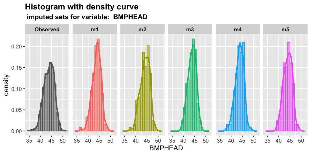

plot_2num(imputation.list = imputed.data, var.x = "BMPHEAD",
    var.y = "BMPRECUM", original.data = withNA.df)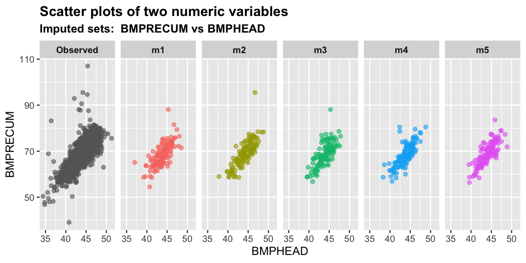

plot_2num(imputation.list = imputed.data, var.x = "HSAGEIR",
    var.y = "BMPHEAD", original.data = withNA.df)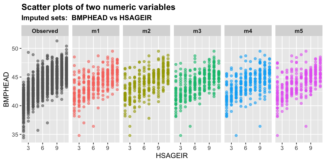

plot_1num1fac(imputation.list = imputed.data, var.num = "BMPHEAD",
    var.fac = "HSSEX", original.data = withNA.df)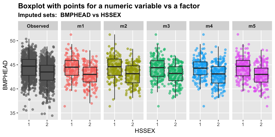

4. Impute new unseen data using a saved imputer object

First we can split the nhanes3_newborn dataset into training data and test data.

library(mixgb)
data("nhanes3_newborn")
set.seed(2022)
n <- nrow(nhanes3_newborn)
idx <- sample(1:n, size = round(0.7 * n), replace = FALSE)
train.data <- nhanes3_newborn[idx, ]
test.data <- nhanes3_newborn[-idx, ]

We can use the training data to obtain m imputed datasets and save their imputation models. To achieve this, users need to set save.models = TRUE. By default save.vars = NULL, imputation models for variables with missing data in the training data will be saved. However, the unseen data may also have missing values in other variables. Users can be comprehensive by saving models for all variables by setting save.vars = colnames(train.data). Note that this would take much longer as we need to train and save a model for each variable. If users are confident that only certain variables will have missing values in the new data, we recommend specifying the names or indices of these variables in save.vars instead of saving models for all variables.

# obtain m imputed datasets for train.data and save
# imputation models
mixgb.obj <- mixgb(data = train.data, m = 5, save.models = TRUE,
    save.vars = NULL)

When save.models = TRUE, mixgb() will return an object containing the following:

• imputed.data: a list of m imputed dataset for training data

• XGB.models: a list of m sets of XGBoost models for variables specified in save.vars.

• params: a list of parameters that are required for imputing new data using impute_new() later on.

We can extract m imputed datasets from the saved imputer object by $imputed.data.

train.imputed <- mixgb.obj$imputed.data
# the 5th imputed dataset
head(train.imputed[[5]])
#>    HSHSIZER HSAGEIR HSSEX DMARACER DMAETHNR DMARETHN BMPHEAD BMPRECUM BMPSB1
#> 1:        7       2     1        1        1        3    43.0     67.1    9.2
#> 2:        4       3     2        2        3        2    42.6     67.1    8.8
#> 3:        3       9     2        2        3        2    46.5     64.3    8.6
#> 4:        3       9     2        1        3        1    46.2     68.5   10.8
#> 5:        5       4     1        1        3        1    44.7     63.0    6.0
#> 6:        5      10     1        1        3        1    45.2     72.0    5.4
#>    BMPSB2 BMPTR1 BMPTR2 BMPWT DMPPIR HFF1 HYD1
#> 1:    8.5    8.8    8.8  7.80  1.701    2    1
#> 2:    8.8   13.3   12.2  8.70  0.102    2    1
#> 3:    8.0   10.4    9.2  8.00  0.359    1    3
#> 4:   10.0   16.6   16.0  8.98  0.561    1    3
#> 5:    5.8    9.0    9.0  7.60  2.379    2    1
#> 6:    5.4    9.2    9.4  9.00  2.173    2    2

To impute new data with this saved imputer object, we use the impute_new() function. User can also specify whether to use new data for initial imputation. By default, initial.newdata = FALSE, we will use the information of training data to initially impute the new data. New data will be imputed with the saved models. This process will be considerably faster as we don’t need to build the imputation models again.

test.imputed <- impute_new(object = mixgb.obj, newdata = test.data)

If PMM is used when we call mixgb(), predicted values of missing entries in the new dataset are matched with donors from training data. Users can also set the number of donors for PMM when imputing new data. By default, pmm.k = NULL , which means the same setting as the training object will be used.

Similarly, users can set the number of imputed datasets m. Note that this value has to be smaller than or equal to the m in mixgb(). If it is not specified, it will use the same m value as the saved object.

test.imputed <- impute_new(object = mixgb.obj, newdata = test.data,
    initial.newdata = FALSE, pmm.k = 3, m = 4)

5. Install mixgb with GPU support

Multiple imputation can be run with GPU support for machines with NVIDIA GPUs. Note that users have to install the R package xgboost with GPU support first.

The xgboost R package pre-built binary on Linux x86_64 with GPU support can be downloaded from the release page https://github.com/dmlc/xgboost/releases/tag/v1.4.0

The package can then be installed by running the following commands:

# Install dependencies
$ R -q -e "install.packages(c('data.table', 'jsonlite'))"

# Install XGBoost
$ R CMD INSTALL ./xgboost_r_gpu_linux.tar.gz

Then users can install package mixgb in R.

devtools::install_github("agnesdeng/mixgb")
library(mixgb)

Users just need to specify tree_method = "gpu_list" in the params list which will then be passed to xgb.params in mixgb(). Other GPU-realted arguments include gpu_id and predictor. By default, gpu_id = 0 and predictor = "auto".

params <- list(max_depth = 6, gamma = 0.1, eta = 0.3, min_child_weight = 1,
    subsample = 1, colsample_bytree = 1, colsample_bylevel = 1,
    colsample_bynode = 1, nthread = 4, tree_method = "gpu_list",
    gpu_id = 0, predictor = "auto")


mixgb.data <- mixgb(data = withNA.df, m = 5, xgb.params = params)