multid provides tools for regularized measurement of multivariate differences between two groups (e.g., sex differences). Regularization via logistic regression variants enables inclusion of large number of correlated variables in the multivariate set while providing k-fold cross-validation and regularization to avoid overfitting (D_regularized -function).
Predictive approach as implemented with regularized methods also allows for examination of group-membership probabilities and their distributions across individuals. In the context of statistical predictions of sex, these distributions are an updated variant to gender-typicality distributions used in gender diagnosticity methodology (Lippa & Connelly, 1990).
Studies in which these methods have been used:
multid also includes functions for testing hypothesis that consider predicting algebraic difference scores as variables. A joint test that focuses on the regression coefficients on the difference score components (minuend and subtrahend) is provided in the structural equation modeling framework (sem_dadas) and multilevel models (ml_dadas). Difference between Absolute Difference and Absolute Sum of the regression coefficients (DADAS) is used for direct test of whether the coefficients can be interpreted as predicting a difference score.
In addition, multid includes various helper functions:
Calculation of variance partition coefficient (i.e., intraclass correlation, ICC) with vpc_at -function at different levels of lower-level predictors in two-level model including random slope (Goldstein et al., 2002)
Calculation of coefficient of variance variation and standardized variance heterogeneity, either with manual input of estimates (cvv_manual) or directly from data (cvv) (Ruscio & Roche, 2012)
Calculation of reliability of difference score variable that is a difference between two mean values (e.g., difference between men and women across countries) by using ICC2 reliability estimates (Bliese, 2000) as inputs in the equation for difference score reliability (Johns, 1981). Can be calculated from long format data file or from lmer-fitted two-level model with reliability_dms -function.
You can install the released version of multid from CRAN with:
install.packages("multid")You can install the development version from GitHub with:
# install.packages("devtools")
devtools::install_github("vjilmari/multid")This example shows how to measure standardized multivariate (both Sepal and Petal dimensions, four variables in total) distance between setosa and versicolor Species in iris dataset.
library(multid)
set.seed(91237)

D.iris<-
  D_regularized(
  data = iris[iris$Species == "setosa" | iris$Species == "versicolor", ],
  mv.vars = c(
    "Sepal.Length", "Sepal.Width",
    "Petal.Length", "Petal.Width"
  ),
  group.var = "Species",
  group.values = c("setosa", "versicolor")
)

round(D.iris$D,2)
#>      n.setosa n.versicolor m.setosa m.versicolor sd.setosa sd.versicolor
#> [1,]       50           50     8.35        -9.38      1.39          2.25
#>      pooled.sd  diff    D
#> [1,]      1.87 17.73 9.49

# Use different partitions of data for regularization and estimation
D.iris_out<-
  D_regularized(
  data = iris[iris$Species == "setosa" |
    iris$Species == "versicolor", ],
  mv.vars = c(
    "Sepal.Length", "Sepal.Width",
    "Petal.Length", "Petal.Width"
  ),
  group.var = "Species",
  group.values = c("setosa", "versicolor"),
  size = 35,
  out = TRUE,
  pred.prob = TRUE,
  prob.cutoffs = seq(0,1,0.25)

)

# print group differences (D)
round(D.iris_out$D,2)
#>      n.setosa n.versicolor m.setosa m.versicolor sd.setosa sd.versicolor
#> [1,]       15           15     7.61        -8.97      1.79          2.35
#>      pooled.sd  diff    D
#> [1,]      2.09 16.59 7.93

# print table of predicted probabilities
D.iris_out$P.table
#>
#>              [0,0.25) [0.25,0.5) [0.5,0.75) [0.75,1]
#>   setosa            0          0          0        1
#> versicolor 1 0 0 0This example first generates artificial multi-group data which are then used as separate data folds in the regularization procedure following separate predictions made for each fold.
# generate data for 10 groups
set.seed(34246)
n1 <- 100
n2 <- 10
d <-
  data.frame(
    sex = sample(c("male", "female"), n1 * n2, replace = TRUE),
    fold = sample(x = LETTERS[1:n2], size = n1 * n2, replace = TRUE),
    x1 = rnorm(n1 * n2),
    x2 = rnorm(n1 * n2),
    x3 = rnorm(n1 * n2)
  )
#'
# Fit and predict with same data
round(D_regularized(
  data = d,
  mv.vars = c("x1", "x2", "x3"),
  group.var = "sex",
  group.values = c("female", "male"),
  fold.var = "fold",
  fold = TRUE,
  rename.output = TRUE
)$D,2)
#>   n.female n.male m.female m.male sd.female sd.male pooled.sd  diff     D
#> A       53     48     0.01  -0.02      0.07    0.06      0.07  0.04  0.53
#> B       56     53     0.00  -0.02      0.07    0.06      0.07  0.02  0.27
#> C       39     56    -0.02  -0.01      0.08    0.06      0.07 -0.01 -0.18
#> D       53     58     0.00  -0.01      0.06    0.06      0.06  0.01  0.17
#> E       44     52     0.00   0.01      0.06    0.07      0.06 -0.01 -0.14
#> F       60     31    -0.01  -0.01      0.06    0.06      0.06 -0.01 -0.10
#> G       56     51    -0.01  -0.03      0.06    0.05      0.06  0.01  0.20
#> H       47     51     0.00  -0.01      0.07    0.07      0.07  0.01  0.14
#> I       42     45     0.02  -0.01      0.07    0.07      0.07  0.03  0.48
#> J       48     57     0.00  -0.01      0.05    0.07      0.06  0.01  0.10
#>   pooled.sd.female pooled.sd.male pooled.sd.total d.sd.total
#> A             0.07           0.06            0.07       0.56
#> B             0.07           0.06            0.07       0.26
#> C             0.07           0.06            0.07      -0.19
#> D             0.07           0.06            0.07       0.16
#> E             0.07           0.06            0.07      -0.14
#> F             0.07           0.06            0.07      -0.10
#> G             0.07           0.06            0.07       0.18
#> H             0.07           0.06            0.07       0.15
#> I             0.07           0.06            0.07       0.49
#> J             0.07           0.06            0.07       0.10
#'

# Different partitions for regularization and estimation for each data fold.

# Request probabilities of correct classification (pcc) and
# area under the receiver operating characteristics (auc) for the output.

round(D_regularized(
  data = d,
  mv.vars = c("x1", "x2", "x3"),
  group.var = "sex",
  group.values = c("female", "male"),
  fold.var = "fold",
  size = 17,
  out = TRUE,
  fold = TRUE,
  rename.output = TRUE,
  pcc = TRUE,
  auc = TRUE
)$D,2)
#>   n.female n.male m.female m.male sd.female sd.male pooled.sd  diff     D
#> A       36     31     0.00  -0.01      0.18    0.15      0.17  0.00  0.03
#> B       39     36    -0.04  -0.04      0.16    0.15      0.15 -0.01 -0.04
#> C       22     39    -0.07   0.01      0.17    0.13      0.15 -0.08 -0.56
#> D       36     41     0.01   0.01      0.14    0.17      0.15  0.00 -0.01
#> E       27     35    -0.07   0.00      0.13    0.11      0.12 -0.07 -0.60
#> F       43     14    -0.04   0.04      0.17    0.17      0.17 -0.08 -0.47
#> G       39     34    -0.03  -0.04      0.12    0.15      0.14  0.01  0.07
#> H       30     34     0.04   0.01      0.16    0.15      0.16  0.03  0.18
#> I       25     28     0.02  -0.03      0.14    0.14      0.14  0.05  0.35
#> J       31     40     0.00   0.00      0.15    0.15      0.15  0.00  0.02
#>   pcc.female pcc.male pcc.total  auc pooled.sd.female pooled.sd.male
#> A       0.56     0.39      0.48 0.49             0.15           0.15
#> B       0.36     0.61      0.48 0.50             0.15           0.15
#> C       0.32     0.46      0.41 0.34             0.15           0.15
#> D       0.53     0.49      0.51 0.49             0.15           0.15
#> E       0.37     0.49      0.44 0.37             0.15           0.15
#> F       0.44     0.36      0.42 0.39             0.15           0.15
#> G       0.38     0.59      0.48 0.53             0.15           0.15
#> H       0.73     0.47      0.59 0.57             0.15           0.15
#> I       0.48     0.64      0.57 0.60             0.15           0.15
#> J       0.55     0.45      0.49 0.52             0.15           0.15
#>   pooled.sd.total d.sd.total
#> A            0.15       0.03
#> B            0.15      -0.04
#> C            0.15      -0.54
#> D            0.15      -0.01
#> E            0.15      -0.48
#> F            0.15      -0.54
#> G            0.15       0.06
#> H            0.15       0.19
#> I            0.15       0.32
#> J 0.15 0.02This example compares a measure of standardized distance between group centroids (Mahalanobis’ D) and a regularized variant provided in the multid-package in small-sample scenario when the distance between group centroids in the population is D = 1.
set.seed(8327482)
# generate data from sixteen correlated (r = .20) variables each with d = .50 difference
#(equals to Mahalanobis' D = 1)
k=16
r=0.2
d=0.5
n=200

# population correlation matrix
cor_mat<-matrix(ncol=k,nrow=k,rep(r,k*k))
diag(cor_mat)<-1

# population difference vector
d_vector<-rep(d,k)

# population Mahalanobis' D is exactly 1

sqrt(t(d_vector) %*% solve(cor_mat) %*% d_vector)
#>      [,1]
#> [1,]    1

# generate data
library(MASS)

male.dat<-
  data.frame(sex="male",
             mvrnorm(n = n/2,
                     mu = 0.5*d_vector,
                     Sigma = cor_mat,empirical = F))

female.dat<-
  data.frame(sex="female",
             mvrnorm(n = n/2,
                     mu = -0.5*d_vector,
                     Sigma = cor_mat,empirical = F))

dat<-rbind(male.dat,female.dat)

# sample Mahalanobis' D

# obtain mean differences

d_vector_sample<-rep(NA,k)

for (i in 1:k){
  d_vector_sample[i]<-mean(male.dat[,i+1]-female.dat[,i+1])

}

# sample pooled covariance matrix (use mean, because equal sample sizes)

cov_mat_sample<-
  (cov(male.dat[,2:17])+cov(female.dat[,2:17]))/2

# calculate sample Mahalanobis' D
sqrt(t(d_vector_sample) %*% solve(cov_mat_sample) %*% d_vector_sample)
#>          [,1]
#> [1,] 1.265318

# calculate elastic net D

D.ela<-
  D_regularized(data=dat,
              mv.vars=paste0("X",1:k),
              group.var = "sex",
              group.values = c("male","female"))

round(D.ela$D,2)
#>      n.male n.female m.male m.female sd.male sd.female pooled.sd diff    D
#> [1,]    100      100   0.54    -0.52    0.86      0.88      0.87 1.06 1.22

# use separate data for regularization and estimation

D.ela_out<-D_regularized(data=dat,
              mv.vars=paste0("X",1:k),
              group.var = "sex",
              group.values = c("male","female"),
              out=T,size = 50,pcc = T, auc=T,pred.prob = T)

round(D.ela_out$D,2)
#>      n.male n.female m.male m.female sd.male sd.female pooled.sd diff    D
#> [1,]     50       50   0.55    -0.33    1.04      0.92      0.99 0.88 0.89
#>      pcc.male pcc.female pcc.total  auc
#> [1,]     0.68       0.68      0.68 0.73

# Table of predicted probabilites
D.ela_out$P.table
#>
#>          [0,0.2) [0.2,0.4) [0.4,0.6) [0.6,0.8) [0.8,1]
#>   female    0.10      0.34      0.32      0.20    0.04
#> male 0.00 0.18 0.26 0.36 0.20This example compares a measure of standardized distance between group centroids (Mahalanobis’ D) and a regularized variant provided in the multid-package in small-sample scenario when the group centroids in the population is are at the same location, D = 0. In this sample, Mahalanobis’ D is measured at D = 0.5, elastic net D with same data used for regularization and estimation at D = 0.35, whereas elastic net D with independent estimation data shows D = 0.
set.seed(8327482)
# generate data from sixteen correlated (r = .20) variables each with d = .00 difference
# (equals to Mahalanobis' D = 0)
k=16
r=0.2
d=0.0
n=200

# population correlation matrix
cor_mat<-matrix(ncol=k,nrow=k,rep(r,k*k))
diag(cor_mat)<-1

# population difference vector
d_vector<-rep(d,k)

# population Mahalanobis' D is exactly 1

sqrt(t(d_vector) %*% solve(cor_mat) %*% d_vector)
#>      [,1]
#> [1,]    0

# generate data

male.dat<-
  data.frame(sex="male",
             mvrnorm(n = n/2,
                     mu = 0.5*d_vector,
                     Sigma = cor_mat,empirical = F))

female.dat<-
  data.frame(sex="female",
             mvrnorm(n = n/2,
                     mu = -0.5*d_vector,
                     Sigma = cor_mat,empirical = F))

dat<-rbind(male.dat,female.dat)

# sample Mahalanobis' D

# obtain mean differences

d_vector_sample<-rep(NA,k)

for (i in 1:k){
  d_vector_sample[i]<-mean(male.dat[,i+1]-female.dat[,i+1])

}

# sample pooled covariance matrix (use mean, because equal sample sizes)

cov_mat_sample<-
  (cov(male.dat[,2:17])+cov(female.dat[,2:17]))/2

# calculate sample Mahalanobis' D
sqrt(t(d_vector_sample) %*% solve(cov_mat_sample) %*% d_vector_sample)
#>           [,1]
#> [1,] 0.5316555

# calculate elastic net D

D.ela.zero<-
  D_regularized(data=dat,
              mv.vars=paste0("X",1:k),
              group.var = "sex",
              group.values = c("male","female"))

round(D.ela.zero$D,2)
#>      n.male n.female m.male m.female sd.male sd.female pooled.sd diff    D
#> [1,]    100      100   0.02    -0.02     0.1       0.1       0.1 0.04 0.35

# use separate data for regularization and estimation

D.ela.zero_out<-
  D_regularized(data=dat,
              mv.vars=paste0("X",1:k),
              group.var = "sex",
              group.values = c("male","female"),
              out=T,size = 50,pcc = T, auc=T,pred.prob = T)

round(D.ela.zero_out$D,2)
#>      n.male n.female m.male m.female sd.male sd.female pooled.sd diff   D
#> [1,]     50       50      0        0       0         0         0    0 NaN
#>      pcc.male pcc.female pcc.total auc
#> [1,]        1          0       0.5 0.5

# Table of predicted probabilites
D.ela.zero_out$P.table
#>
#>          [0,0.2) [0.2,0.4) [0.4,0.6) [0.6,0.8) [0.8,1]
#>   female       0         0         1         0       0
#> male 0 0 1 0 0This example shows how the degree of overlap between the predicted values across the two groups can be visualized and estimated.
For parametric variants, see Del Giudice (in press).
For non-parametric variants, see Pastore (2018) and Pastore & Calcagnì (2019).
# Use predicted values from elastic net D (out) when difference in population exists-

library(ggplot2)

ggplot(D.ela_out$pred.dat,
       aes(x=pred,fill=group))+
  geom_density(alpha=0.5)+
  xlab("Predicted log odds of being male (FM-score)")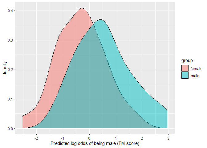
# parametric overlap

## Proportion of overlap relative to a single distribution (OVL)

## obtain D first
(D<-unname(D.ela_out$D[,"D"]))
#> [1] 0.8884007

(OVL<-2*pnorm((-D/2)))
#> [1] 0.6568977

## Proportion of overlap relative to the joint distribution

(OVL2<-OVL/(2-OVL))
#> [1] 0.4890899

# non-parametric overlap

library(overlapping)

np.overlap<-
  overlap(x = list(D.ela_out$pred.dat[
  D.ela_out$pred.dat$group=="male","pred"],
  D.ela_out$pred.dat[
  D.ela_out$pred.dat$group=="female","pred"]),
  plot=T)
# this corresponds to Proportion of overlap relative to the joint distribution (OVL2)
(np.OVL2<-unname(np.overlap$OV))
#> [1] 0.5412493

# from which Proportion of overlap relative to a single distribution (OVL) is approximated at
(np.OVL<-(2*np.OVL2)/(1+np.OVL2))
#> [1] 0.7023514

# compare overlaps

round(cbind(OVL,np.OVL,OVL2,np.OVL2),2)
#>       OVL np.OVL OVL2 np.OVL2
#> [1,] 0.66 0.7 0.49 0.54# sem example
set.seed(342356)
d <- data.frame(
var1 = rnorm(50),
var2 = rnorm(50),
x = rnorm(50)
)
round(sem_dadas(
data = d, var1 = "var1", var2 = "var2",
predictor = "x", center = TRUE, scale = TRUE
)$results,3)
#> est se z pvalue ci.lower ci.upper
#> b_11 0.107 0.143 0.747 0.455 -0.174 0.388
#> b_21 -0.078 0.110 -0.710 0.477 -0.294 0.138
#> b_10 -0.031 0.151 -0.205 0.837 -0.327 0.265
#> b_20 0.031 0.127 0.244 0.807 -0.218 0.280
#> rescov_12 -0.153 0.140 -1.096 0.273 -0.428 0.121
#> coef_diff 0.185 0.196 0.943 0.346 -0.200 0.570
#> coef_diff_std 0.120 0.125 0.960 0.337 -0.125 0.365
#> coef_sum 0.029 0.163 0.176 0.860 -0.291 0.349
#> diff_abs_magnitude 0.029 0.163 0.176 0.860 -0.291 0.349
#> abs_coef_diff 0.185 0.196 0.943 0.173 -0.200 0.570
#> abs_coef_sum 0.029 0.163 0.176 0.430 -0.291 0.349
#> dadas 0.157 0.220 0.710 0.239 -0.275 0.588
# multilevel example
set.seed(95332)
n1 <- 10 # groups
n2 <- 10 # observations per group
dat <- data.frame(
group = rep(c(LETTERS[1:n1]), each = n2),
x = sample(c(-0.5, 0.5), n1 * n2, replace = TRUE),
w = rep(sample(1:5, n1, replace = TRUE), each = n2),
y = sample(1:5, n1 * n2, replace = TRUE)
)
library(lmerTest)
fit <- lmerTest::lmer(y ~ x * w + (x | group),
data = dat
)
round(ml_dadas(fit,
predictor = "w",
diff_var = "x",
diff_var_values = c(0.5, -0.5))$dadas, 3)
#> estimate SE df t.ratio p.value
#> -0.5 -0.077 0.177 8.053 -0.435 0.675
#> 0.5 -0.279 0.136 9.326 -2.048 0.070
#> abs_diff 0.202 0.228 7.071 0.886 0.202
#> abs_sum 0.356 0.219 6.952 1.630 0.074
#> dadas -0.154 0.354 8.053 -0.435 0.662