An R package for ordinal pattern analysis.
opa can be installed from CRAN with:
install.packages("opa")You can install the development version of opa from GitHub with:
# install.packages("remotes")
remotes::install_github("timbeechey/opa")To cite opa in your work you can use the output of:
citation(package = "opa")opa is an implementation of methods described in
publications including Thorngate
(1987) and (Grice
et al., 2015). Thorngate (1987) attributes the original idea to:
Parsons, D. (1975). The directory of tunes and musical themes. S. Brown.
Ordinal pattern analysis is similar to Kendall’s Tau. Whereas Kendall’s tau is a measure of similarity between two data sets in terms of rank ordering, ordinal pattern analysis is intended to quantify the match between an hypothesis and patterns of individual-level data across conditions or mesaurement instances.
Ordinal pattern analysis works by comparing the relative ordering of pairs of observations and computing whether these pairwise relations are matched by an hypothesis. Each pairwise ordered relation is classified as an increases, a decrease, or as no change. These classifications are encoded as 1, -1 and 0, respectively. An hypothesis of a monotonic increase in the response variable across four experimental conditions can be specified as:
h <- c(1, 2, 3, 4)The hypothesis h encodes six pairwise relations, all
increases: 1 1 1 1 1 1.
A row of individual data representing measurements across four conditions, such as:
dat <- c(65.3, 68.8, 67.0, 73.1)encodes the ordered pairwise relations 1 1 1 -1 1 1. The
percentage of orderings which are correctly classified by the hypothesis
(PCC) is the main quantity of interest in ordinal pattern analysis.
Comparing h and dat, the PCC is
5/6 = 0.833 or 83.3%. An hypothesis which generates a
greater PCC is preferred over an hypothesis which generates a lower PCC
for given data.
It is also possible to calculate a chance-value for a PCC which is equal to the chance that a PCC at least as great as the PCC of the observed data could occur as a result of a random ordering of the data. Chance values can be computed using either a permutation test or a randomization test.
opalibrary(opa)A hypothesized relative ordering of the response variable across conditions is specified with a numeric vector:
h <- c(1, 2, 4, 3)The hypothesis can be visualized with the
plot_hypothesis() function:
plot_hypothesis(h)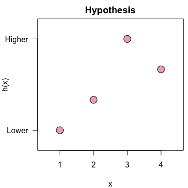
Data should be in wide format with one column per measurement condition and one row per individual:
set.seed(123)

dat <- data.frame(t1 = rnorm(20, mean = 12, sd = 2),
                  t2 = rnorm(20, mean = 15, sd = 2),
                  t3 = rnorm(20, mean = 20, sd = 2),
                  t4 = rnorm(20, mean = 17, sd = 2))

round(dat, 2)
#>       t1    t2    t3    t4
#> 1  10.88 12.86 18.61 17.76
#> 2  11.54 14.56 19.58 16.00
#> 3  15.12 12.95 17.47 16.33
#> 4  12.14 13.54 24.34 14.96
#> 5  12.26 13.75 22.42 14.86
#> 6  15.43 11.63 17.75 17.61
#> 7  12.92 16.68 19.19 17.90
#> 8   9.47 15.31 19.07 17.11
#> 9  10.63 12.72 21.56 18.84
#> 10 11.11 17.51 19.83 21.10
#> 11 14.45 15.85 20.51 16.02
#> 12 12.72 14.41 19.94 12.38
#> 13 12.80 16.79 19.91 19.01
#> 14 12.22 16.76 22.74 15.58
#> 15 10.89 16.64 19.55 15.62
#> 16 15.57 16.38 23.03 19.05
#> 17 13.00 16.11 16.90 16.43
#> 18  8.07 14.88 21.17 14.56
#> 19 13.40 14.39 20.25 17.36
#> 20 11.05 14.24 20.43 16.72
An ordinal pattern analysis model to consider how the hypothesis
h matches each individual pattern of results in
dat can be fitted using:
opamod <- opa(dat, h, cval_method = "exact")A summary of the model output can be viewed using:
summary(opamod)
#> Ordinal Pattern Analysis of 4 observations for 20 individuals in 1 group
#>
#> Between subjects results:
#>          PCC cval
#> pooled 93.33  0.1
#>
#> Within subjects results:
#>       PCC cval
#> 1  100.00 0.04
#> 2  100.00 0.04
#> 3   83.33 0.17
#> 4  100.00 0.04
#> 5  100.00 0.04
#> 6   83.33 0.17
#> 7  100.00 0.04
#> 8  100.00 0.04
#> 9  100.00 0.04
#> 10  83.33 0.17
#> 11 100.00 0.04
#> 12  66.67 0.38
#> 13 100.00 0.04
#> 14  83.33 0.17
#> 15  83.33 0.17
#> 16 100.00 0.04
#> 17 100.00 0.04
#> 18  83.33 0.17
#> 19 100.00 0.04
#> 20 100.00 0.04
#>
#> PCCs were calculated for pairwise ordinal relationships using a difference threshold of 0.
#> Chance-values were calculated using the exact method.
Individual-level model output can be visualized using:
plot(opamod)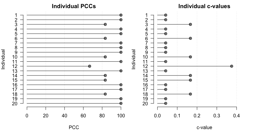
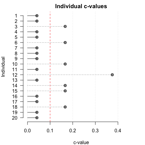
To aid in visual interpretation, iIndividual PCCs and c-values can also be plotted relative to specified thresholds:
pcc_plot(opamod, threshold = 90)
cval_plot(opamod, threshold = 0.1)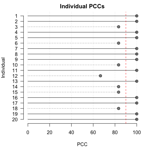
Pairwise comparisons of measurement conditions can be calculated by
applying the compare_conditions() function to an
opafit object produced by a call to opa():
condition_comparisons <- compare_conditions(opamod)

condition_comparisons$pccs
#>     1   2  3 4
#> 1   -   -  - -
#> 2  90   -  - -
#> 3 100 100  - -
#> 4  95  80 95 -
condition_comparisons$cvals
#>       1   2     3 4
#> 1     -   -     - -
#> 2  0.55   -     - -
#> 3   0.5 0.5     - -
#> 4 0.525 0.6 0.525 -If the data consist of multiple groups a categorical grouping
variable can be passed with the group keyword to produce
results for each group within the data, in addition to individual
results.
dat$group <- rep(c("A", "B", "C", "D"), 5)
dat$group <- factor(dat$group, levels = c("A", "B", "C", "D"))

opamod2 <- opa(dat[, 1:4], h, group = dat$group, cval_method = "exact")
The summary output displays results organised by group.
summary(opamod2)
#> Ordinal Pattern Analysis of 4 observations for 20 individuals in 4 groups
#>
#> Between subjects results:
#>      PCC cval
#> A 100.00 0.04
#> B  86.67 0.14
#> C  93.33 0.09
#> D  93.33 0.11
#>
#> Within subjects results:
#>   Individual    PCC cval
#> A          1 100.00 0.04
#> A          5 100.00 0.04
#> A          9 100.00 0.04
#> A         13 100.00 0.04
#> A         17 100.00 0.04
#> B          2 100.00 0.04
#> B          6  83.33 0.17
#> B         10  83.33 0.17
#> B         14  83.33 0.17
#> B         18  83.33 0.17
#> C          3  83.33 0.17
#> C          7 100.00 0.04
#> C         11 100.00 0.04
#> C         15  83.33 0.17
#> C         19 100.00 0.04
#> D          4 100.00 0.04
#> D          8 100.00 0.04
#> D         12  66.67 0.38
#> D         16 100.00 0.04
#> D         20 100.00 0.04
#>
#> PCCs were calculated for pairwise ordinal relationships using a difference threshold of 0.
#> Chance-values were calculated using the exact method.
Similarly, plotting the output shows individual PCCs and c-values by group.
plot(opamod2)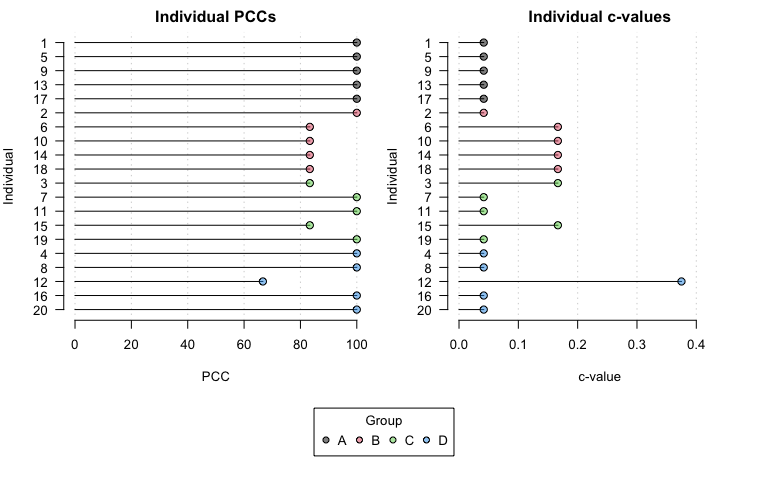
Development of opa was supported by a Medical Research
Foundation Fellowship (MRF-049-0004-F-BEEC-C0899).