optimLanduse provides methods for robust multi-criterial landscape optimization that explicitly account for uncertainty in the optimization of the land allocation to land-use options. High landscape diversity is assumed to increase the number and level of ecosystem services. However, the interactions between ecosystem service provision, disturbances and landscape composition are poorly understood. Knoke et al. (2016) therefore presented a novel approach to incorporate uncertainty in land allocation optimization to improve the provision of multiple ecosystem services. The optimization framework of Knoke et al. (2016) is implemented in the optimLanduse package, aiming to make it easily accessible for practical land-use optimization and to enable efficient batch applications.
The method is already established in land-use optimization and has been applied in a couple of studies. More details about the theory, the definition of the formal optimization problem and also significant examples are listed in the literature section
We designed a graphical shiny application for the package to get a quick idea of the functionalities of the package, see https://gitlab.gwdg.de/forest_economics_goettingen/optimlanduse_shiny.
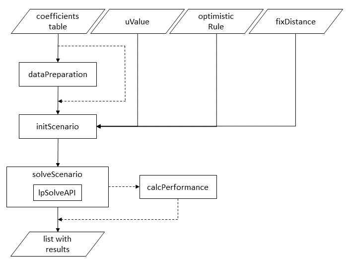
This chapter provides brief overview over the package functions. Please consider their respective help pages for more information. The function lpSolveAPI comes from the lpSolveAPI package. https://cran.r-project.org/package=lpSolveAPI
An optimLanduse object containing informations of the optimization model and solution. It contains among others the - land use allocation in the optimum, - the detailed table with all possible indicator combinations (the scenario table), and the - minimum distance β.
Install package
Simple example
require(readxl)
library(optimLanduse)

path <- exampleData("exampleGosling.xlsx")
dat <- read_excel(path)

init <- initScenario(dat,
                     uValue = 2,
                     optimisticRule = "expectation",
                     fixDistance = 3)
result <- solveScenario(x = init)
performance <- calcPerformance(result)


result$landUse
result$scenarioTable
result$scenarioSettings
result$status
result$beta
Exemplary batch application for distinct uncertainty values u
require(readxl)
library(optimLanduse)

path <- exampleData("exampleGosling.xlsx")
dat <- read_excel(path)

# define sequence of uncertainties
u <- seq(1, 5, 1)

# prepare empty data frame for the results

## alternative 1: loop, simply implemented ##

loopDf <- data.frame(u = u, matrix(NA, nrow = length(u), ncol = 1 + length(unique(dat$landUse))))
names(loopDf) <- c("u", "beta", unique(dat$landUse))

for(i in u) {
  init <- initScenario(dat, uValue = i, optimisticRule = "expectation", fixDistance = 3)
  result <- solveScenario(x = init)
  loopDf[loopDf$u == i,] <- c(i, result$beta, as.matrix(result$landUse))
}

# alternative 2: apply, faster
applyDf <- data.frame(u = u)

applyFun <- function(x) {
  init <- initScenario(dat, uValue = x, optimisticRule = "expectation", fixDistance = 3)
  result <- solveScenario(x = init)
  return(c(result$beta, as.matrix(result$landUse)))
}

applyDf <- cbind(applyDf,
                 t(apply(applyDf, 1, applyFun)))

names(applyDf) <- c("u", "beta", names(result$landUse))
Plot the land-use allocations with increasing uncertainty
# Typical result visualization
require(ggplot2)
require(dplyr)
require(tidyr)

applyDf %>% gather(key = "land-use option", value = "land-use share", -u, -beta) %>%
  ggplot(aes(y = `land-use share`, x = u, fill = `land-use option`)) +
  geom_area(alpha = .8, color = "white") + theme_minimal()
Batch example - parallel
library(optimLanduse)
require(readxl)
require(foreach)
require(doParallel)

path <- exampleData("exampleGosling.xlsx")
dat <- read_excel(path)

registerDoParallel(8)

u <- seq(1, 5, 1)


loopDf1 <- foreach(i = u, .combine = rbind, .packages = "optimLanduse") %dopar% {
  init <- initScenario(dat, uValue = i, optimisticRule = "expectation", fixDistance = 3)
  result <- solveScenario(x = init)
  c(i, result$beta, as.matrix(result$landUse))
}

stopImplicitCluster()Gosling, E., Reith, E., Knoke T., Gerique, A., Paul, C. (2020): Exploring farmer perceptions of agroforestry via multi-objective optimisation: a test application in Eastern Panama. Agroforestry Systems 94(5). https://doi.org/10.1007/s10457-020-00519-0
Knoke, T., Paul, C., Hildebrandt, P. et al. (2016): Compositional diversity of rehabilitated tropical lands supports multiple ecosystem services and buffers uncertainties. Nat Commun 7, 11877. https://doi.org/10.1038/ncomms11877
Paul, C., Weber, M., Knoke, T. (2017): Agroforestry versus farm mosaic systems – Comparing land-use efficiency, economic returns and risks under climate change effects. Sci. Total Environ. 587-588. https://doi.org/10.1016/j.scitotenv.2017.02.037.
Knoke, T., Paul, C., et al. (2020). Accounting for multiple ecosystem services in a simulation of land‐use decisions: Does it reduce tropical deforestation?. Global change biology 26(4). https://doi.org/10.1111/gcb.15003