‘packageRank’
is an R package that helps put package download counts into context. It
does so via two core functions, cranDownloads() and
packageRank(), a set of filters that reduces package
download count inflation, and other assorted functions that help you
assess interest in your package.
I discuss these topics in four sections; a fifth discusses package related issues.
cranDownloads() extends the
functionality of cranlogs::cran_downloads()
by adding a more user-friendly interface and by providing a generic R
plot() method that makes visualization easy.packageRank() uses rank percentiles, a nonparametric
statistic that tells you the percentage of packages with fewer
downloads, to help you see how your package is doing relative to
all other CRAN
packages.logInfo();
and the internet connection time out problem.To install ‘packageRank’ from CRAN:
install.packages("packageRank")To install the development version from GitHub:
# You may need to first install 'remotes' via install.packages("remotes").
remotes::install_github("lindbrook/packageRank", build_vignettes = TRUE)
Note that ‘packageRank’ has two sets of online upstream dependencies: 1) RStudio’s CRAN package download logs, which records traffic to the “0-Cloud” mirror at cloud.r-project.org (formerly RStudio’s CRAN mirror); and 2) Gábor Csárdi’s ‘cranlogs’ R package, which is an interface to a database that computes R and R package download counts using the aforementioned logs.
When everything is working right, the CRAN package download logs for the previous day will be posted by 17:00 UTC and the results for ‘cranlogs’ will be available soon after.
However, occasionally problems with “today’s” data can emerge due to the downstream nature of the dependencies (illustrated below).
CRAN Download Logs --> 'cranlogs' --> 'packageRank'If there’s a problem with the logs (e.g., they’re not posted on time), both ‘cranlogs’ and ‘packageRank’ will be affected. Here, you’ll see things like an unexpected zero count(s) for your package(s) (actually, it’ll be zero downloads for all of CRAN), data from “yesterday”, or a “Log is not (yet) on the server” error message.
'cranlogs' --> packageRank::cranDownloads()If there’s a problem with ‘cranlogs’ but
not with the logs, only
packageRank::cranDownalods() will be affected (the zero
downloads problem). All the other ‘packageRank’
functions should work since they directly access the logs or other
sources.
Usually, these errors resolve themselves when the underlying scripts
are run (“tomorrow”, if not sooner). For more details, see the “time
zones and logInfo()” section in V
Notes.
cranDownloads() uses all the same arguments as
cranlogs::cran_downloads():
cranlogs::cran_downloads(packages = "HistData")> date count package
> 1 2020-05-01 338 HistDataThe only difference is that cranDownloads() adds four
features:
cranDownloads(packages = "GGplot2")## Error in cranDownloads(packages = "GGplot2") :
## GGplot2: misspelled or not on CRAN.cranDownloads(packages = "ggplot2")> date count cumulative package
> 1 2020-05-01 56357 56357 ggplot2
This also works for inactive or “retired” packages in the Archive:
cranDownloads(packages = "vr")## Error in cranDownloads(packages = "vr") :
## vr: misspelled or not on CRAN/Archive.cranDownloads(packages = "VR")> date count cumulative package
> 1 2020-05-01 11 11 VRWith cranlogs::cran_downloads(), you specify a time
frame using the from and to arguments. The
downside of this is that you must use the “yyyy-mm-dd” date
format. For convenience’s sake, cranDownloads() also allows
you to use “yyyy-mm” or yyyy (“yyyy” also works).
Let’s say you want the download counts for ‘HistData’ for
February 2020. With cranlogs::cran_downloads(), you’d have
to type out the whole date and remember that 2020 was a leap year:
cranlogs::cran_downloads(packages = "HistData", from = "2020-02-01",
  to = "2020-02-29")
With cranDownloads(), you can just specify the
year and month:
cranDownloads(packages = "HistData", from = "2020-02", to = "2020-02")Let’s say you want the download counts for ‘rstan’ for 2020.
With cranlogs::cran_downloads(), you’d type something
like:
cranlogs::cran_downloads(packages = "rstan", from = "2022-01-01",
  to = "2022-12-31")
With cranDownloads(), you can use:
cranDownloads(packages = "rstan", from = 2020, to = 2020)or
cranDownloads(packages = "rstan", from = "2020", to = "2020")from = and to = in
cranDownloads()These additional date formats help to create convenient shortcuts.
Let’s say you want the year-to-date download counts for ‘rstan’. With
cranlogs::cran_downloads(), you’d type something like:
cranlogs::cran_downloads(packages = "rstan", from = "2022-01-01",
  to = Sys.Date() - 1)
With cranDownloads(), you can just pass the
current year to from =:
cranDownloads(packages = "rstan", from = 2022)And if you wanted the entire download history, pass the current year
to to =:
cranDownloads(packages = "rstan", to = 2022)Note that because the RStudio logs begin on 01 October 2012, download data for packages published before that date are unavailable.
cranDownloads(packages = "HistData", from = "2019-01-15",
  to = "2019-01-35")
## Error in resolveDate(to, type = "to") : Not a valid date.cranDownloads(packages = "HistData", when = "last-week")> date count cumulative package
> 1 2020-05-01 338 338 HistData
> 2 2020-05-02 259 597 HistData
> 3 2020-05-03 321 918 HistData
> 4 2020-05-04 344 1262 HistData
> 5 2020-05-05 324 1586 HistData
> 6 2020-05-06 356 1942 HistData
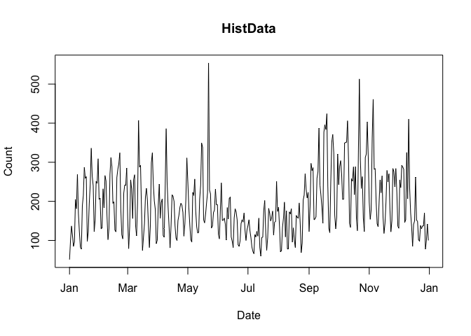
> 7 2020-05-07 324 2266 HistDatacranDownloads() makes visualizing package downloads
easy. Just use plot():
plot(cranDownloads(packages = "HistData", from = "2019", to = "2019"))
If you pass a vector of package names for a single day,
plot() returns a dotchart:
plot(cranDownloads(packages = c("ggplot2", "data.table", "Rcpp"),
  from = "2020-03-01", to = "2020-03-01"))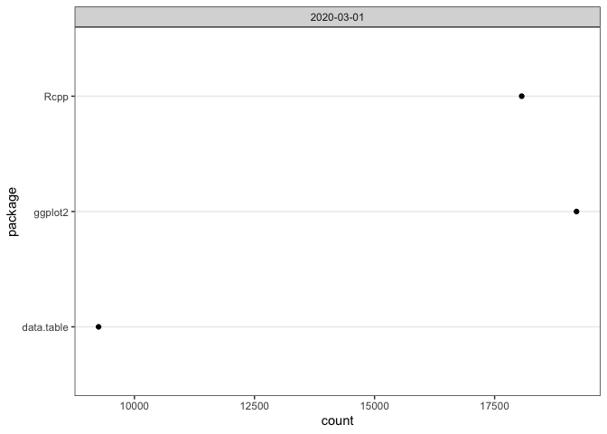
If you pass a vector of package names for multiple days,
plot() uses ‘ggplot2’
facets:
plot(cranDownloads(packages = c("ggplot2", "data.table", "Rcpp"),
  from = "2020", to = "2020-03-20"))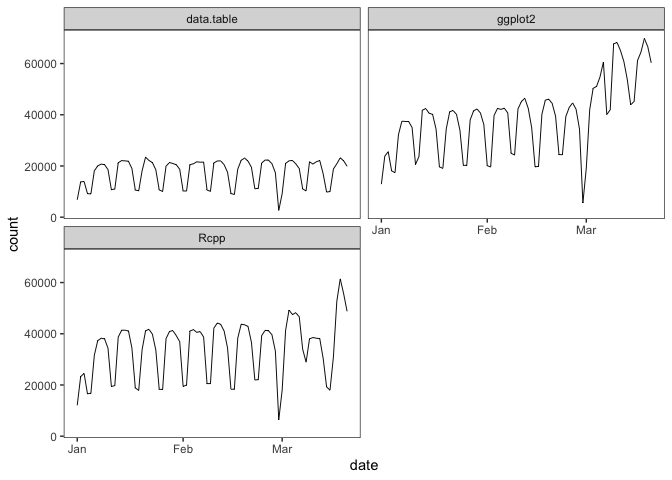
If you want to plot those data in a single frame, set
multi.plot = TRUE:
plot(cranDownloads(packages = c("ggplot2", "data.table", "Rcpp"),
  from = "2020", to = "2020-03-20"), multi.plot = TRUE)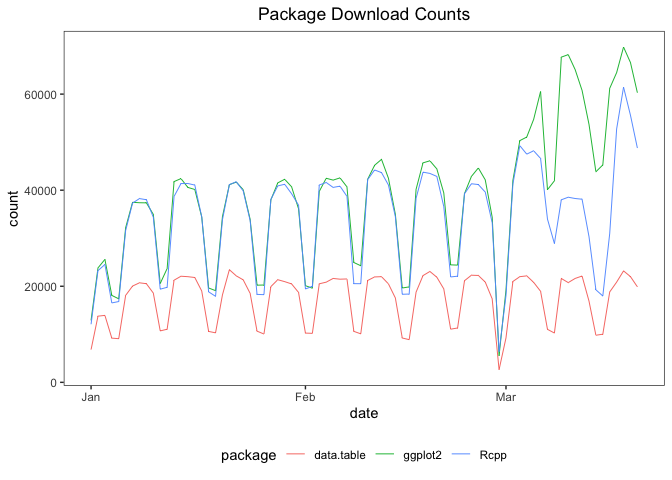
If you want plot those data in separate plots but use the same
scale, set graphics = "base" and you’ll be prompted for
each plot:
plot(cranDownloads(packages = c("ggplot2", "data.table", "Rcpp"),
  from = "2020", to = "2020-03-20"), graphics = "base")
If you want do the above but on separate independent scales, set
same.xy = FALSE:
plot(cranDownloads(packages = c("ggplot2", "data.table", "Rcpp"),
from = "2020", to = "2020-03-20"), graphics = "base", same.xy = FALSE)To use the base 10 logarithm of the download count in a plot, set
log.y = TRUE:
plot(cranDownloads(packages = "HistData", from = "2019", to = "2019"),
  log.y = TRUE)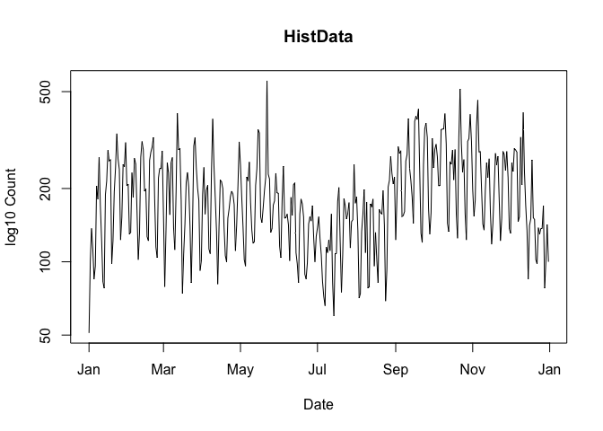
Note that for the sake of the plot, zero counts are replaced by ones
so that the logarithm can be computed. This does not affect the data
returned by cranDownloads().
packages = NULLcranlogs::cran_download(packages = NULL) computes the
total number of package downloads from CRAN. You can plot these data by
using:
plot(cranDownloads(from = 2019, to = 2019))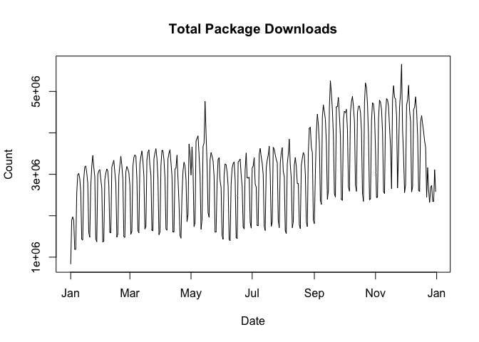
packages = "R"cranlogs::cran_download(packages = "R") computes the
total number of downloads of the R application (note that you can only
use “R” or a vector of packages names, not both!). You can plot these
data by using:
plot(cranDownloads(packages = "R", from = 2019, to = 2019))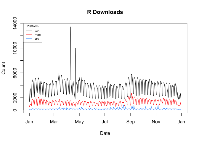
If you want the total count of R downloads, set
r.total = TRUE:
plot(cranDownloads(packages = "R", from = 2019, to = 2019), r.total = TRUE)To add a lowess smoother to your plot, use
smooth = TRUE:
plot(cranDownloads(packages = "rstan", from = "2019", to = "2019"),
  smooth = TRUE)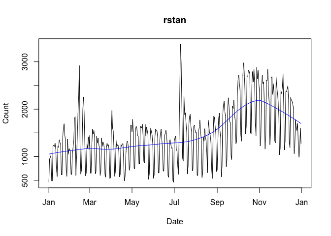
With graphs that use ‘ggplot2’, se = TRUE will add
confidence intervals:
plot(cranDownloads(packages = c("HistData", "rnaturalearth", "Zelig"),
  from = "2020", to = "2020-03-20"), smooth = TRUE, se = TRUE)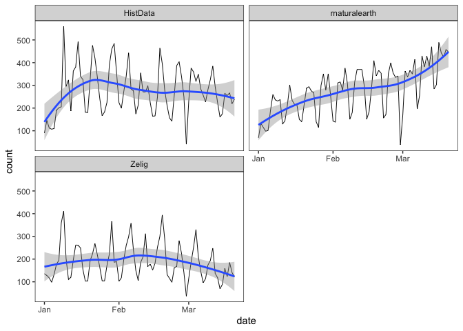
To annotate a graph with a package’s release dates:
plot(cranDownloads(packages = "rstan", from = "2019", to = "2019"),
  package.version = TRUE)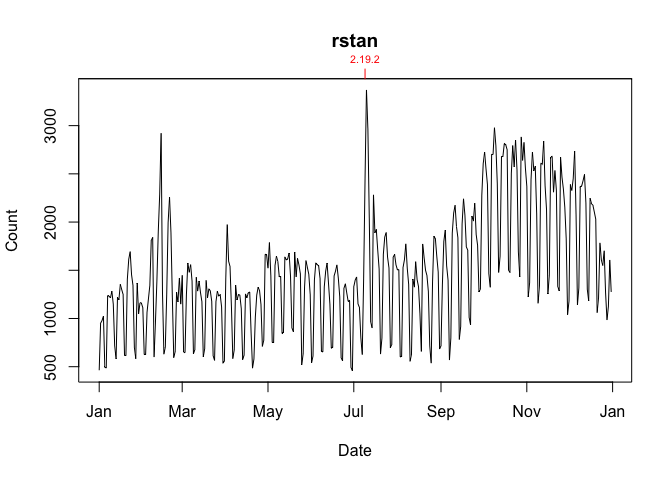
To annotate a graph with R release dates:
plot(cranDownloads(packages = "rstan", from = "2019", to = "2019"),
  r.version = TRUE)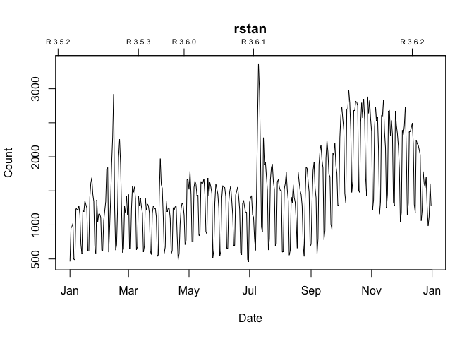
To plot growth curves, set statistic = "cumulative":
plot(cranDownloads(packages = c("ggplot2", "data.table", "Rcpp"),
  from = "2020", to = "2020-03-20"), statistic = "cumulative",
  multi.plot = TRUE, points = FALSE)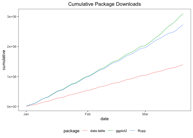
To visualize a package’s downloads relative to “all” other packages over time:
plot(cranDownloads(packages = "HistData", from = "2020", to = "2020-03-20"),
  population.plot = TRUE)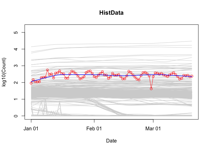
This longitudinal view of package downloads plots the date (x-axis) against the base 10 logarithm of the selected package’s downloads (y-axis). To get a sense of how the selected package’s performance stacks up against all other packages, a set of smoothed curves representing a stratified random sample of packages is plotted in gray in the background (the “typical” pattern of downloads on CRAN for the selected time period). Specifically, within each 5% interval of rank percentiles (e.g., 0 to 5, 5 to 10, 95 to 100, etc.), a random sample of 5% of packages is selected and tracked.
The unit of observation for both cranDownloads() and
cranlogs::cran_dowanlods() is the “day”. The graph below
plots the daily downloads for ‘cranlogs’ from
01 January 2022 through 15 April 2022.
plot(cranDownloads(packages = "cranlogs", from = 2022, to = "2022-04-15"))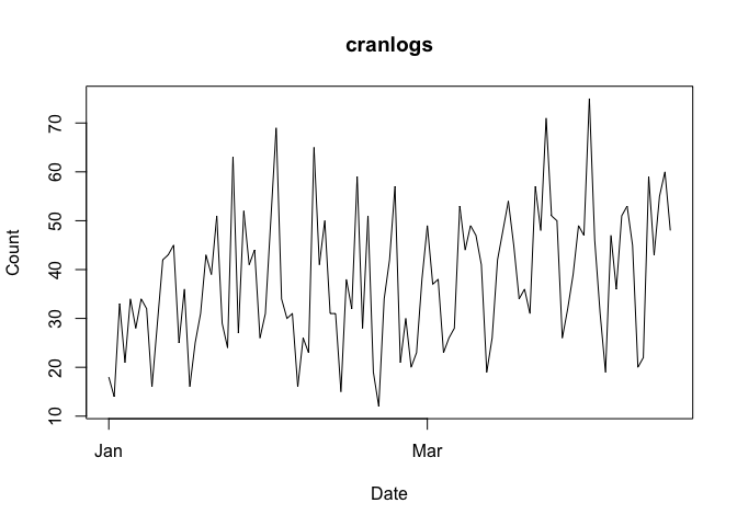
To view the data from a less granular perspective, set
plot.cranDownloads()’s unit.observation argument to “week”,
“month”, or “year”.
unit.observation = "month"The graph below plots the data aggregated by month (with an added smoother):
plot(cranDownloads(packages = "cranlogs", from = 2022, to = "2022-04-15"),
  unit.observation = "month", smooth = TRUE, graphics = "ggplot2")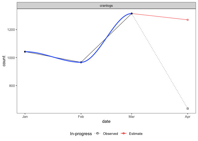
Three things to note. First, if the last/current month (far right) is still in-progress (it’s not the end of the month), that observation will be split in two: one point for the in-progress total (empty black square), another for the estimated total (empty red circle). The estimate is based on the proportion of the month completed. In the example above, the 635 observed downloads from April 1 through April 15 translates into an estimate of 1,270 downloads for the entire month (30 / 15 * 635). Second, if a smoother is included, it will only use “complete”, not in-progress or estimated data. Third, all points are plotted along the x-axis on the first day of the month.
unit.observation = "week"The graph below plots the data aggregated by week (weeks begin on Sunday).
plot(cranDownloads(packages = "cranlogs", from = 2022, to = "2022-06-15"),
    unit.observation = "week", smooth = TRUE)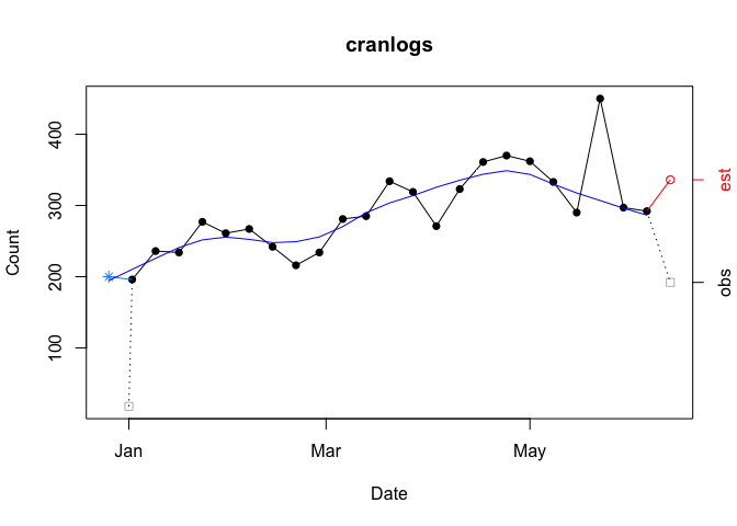
Four things to note. First, if the first week (far left) is incomplete (the ‘from’ date is not a Sunday), that observation will be split in two: one point for the observed total on the nominal start date (gray empty square) and another point for the backdated total. Backdating involves completing the week by pushing the nominal start date back to include the previous Sunday (blue asterisk). In the example above, the nominal start date (01 January 2022) is moved back to include data through the previous Sunday (26 December 2021). This is useful because with a weekly unit of observation the first observation is likely to be truncated and would not give the most representative picture of the data. Second, if the last week (far right) is in-progress (the ‘to’ date is not a Saturday), that observation will be split in two: the observed total (gray empty square) and the estimated total based on the proportion of week completed (red empty circle). Third, just like the monthly plot, smoothers only use complete data, including backdated data but excluding in-progress and estimated data. Fourth, with the exception of first week’s observed count, which is plotted at its nominal date, points are plotted along the x-axis on Sundays, the first day of the week.
After spending some time with nominal download counts, the “compared to what?” question will come to mind. For instance, consider the data for the ‘cholera’ package from the first week of March 2020:
plot(cranDownloads(packages = "cholera", from = "2020-03-01",
  to = "2020-03-07"))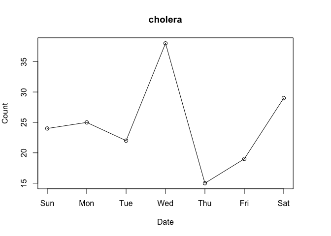
Do Wednesday and Saturday reflect surges of interest in the package or surges of traffic to CRAN? To put it differently, how can we know if a given download count is typical or unusual? One way to answer these questions is to locate your package in the overall frequency distribution of download counts.
Below are the distributions of logarithm of download counts for Wednesday and Saturday. Each vertical segment (along the x-axis) represents a download count. The height of a segment represents that download count’s frequency. The location of ‘cholera’ in the distribution is highlighted in red.
plot(packageDistribution(package = "cholera", date = "2020-03-04"))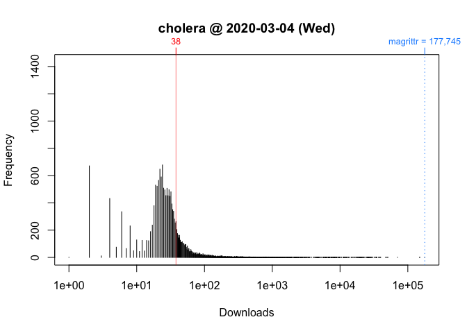
plot(packageDistribution(package = "cholera", date = "2020-03-07"))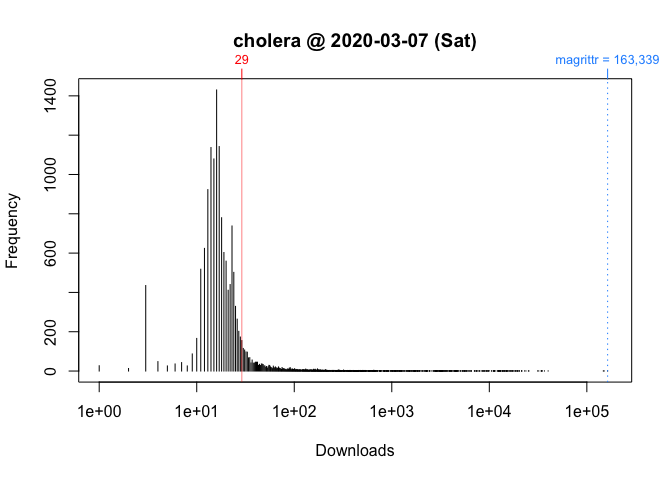
While these plots give us a better picture of where ‘cholera’ is located, comparisons between Wednesday and Saturday are impressionistic at best: all we can confidently say is that the download counts for both days were greater than the mode.
To facilitate interpretation and comparison, I use the rank percentile of a download count instead of the simple nominal download count. This nonparametric statistic tells you the percentage of packages that had fewer downloads. In other words, it gives you the location of your package relative to the locations of all other packages. More importantly, by rescaling download counts to lie on the bounded interval between 0 and 100, rank percentiles make it easier to compare packages within and across distributions.
For example, we can compare Wednesday (“2020-03-04”) to Saturday (“2020-03-07”):
packageRank(package = "cholera", date = "2020-03-04")
>         date packages downloads            rank percentile
> 1 2020-03-04  cholera        38 5,556 of 18,038       67.9
On Wednesday, we can see that ‘cholera’ had 38 downloads, came in 5,556th place out of the 18,038 different packages downloaded, and earned a spot in the 68th percentile.
packageRank(package = "cholera", date = "2020-03-07")
>         date packages downloads            rank percentile
> 1 2020-03-07  cholera        29 3,061 of 15,950         80
On Saturday, we can see that ‘cholera’ had 29 downloads, came in 3,061st place out of the 15,950 different packages downloaded, and earned a spot in the 80th percentile.
So contrary to what the nominal counts tell us, one could say that the interest in ‘cholera’ was actually greater on Saturday than on Wednesday.
To compute rank percentiles, I do the following. For each package, I tabulate the number of downloads and then compute the percentage of packages with fewer downloads. Here are the details using ‘cholera’ from Wednesday as an example:
pkg.rank <- packageRank(packages = "cholera", date = "2020-03-04")

downloads <- pkg.rank$freqtab

round(100 * mean(downloads < downloads["cholera"]), 1)
> [1] 67.9
To put it differently:
(pkgs.with.fewer.downloads <- sum(downloads < downloads["cholera"]))
> [1] 12250

(tot.pkgs <- length(downloads))
> [1] 18038

round(100 * pkgs.with.fewer.downloads / tot.pkgs, 1)
> [1] 67.9In the example above, 38 downloads puts ‘cholera’ in 5,556th place among 18,038 observed packages. This rank is “nominal” because it’s possible that multiple packages can have the same number of downloads. As a result, a package’s nominal rank but not its rank percentile can be affected by its name. For example, because packages with the same number of downloads are sorted in alphabetical order, ‘cholera’ benefits from the fact that it is 31st in the list of 263 packages with 38 downloads:
pkg.rank <- packageRank(packages = "cholera", date = "2020-03-04")
downloads <- pkg.rank$freqtab

which(names(downloads[downloads == 38]) == "cholera")
> [1] 31
length(downloads[downloads == 38])
> [1] 263To visualize packageRank(), use plot().
plot(packageRank(packages = "cholera", date = "2020-03-04"))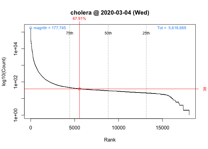
plot(packageRank(packages = "cholera", date = "2020-03-07"))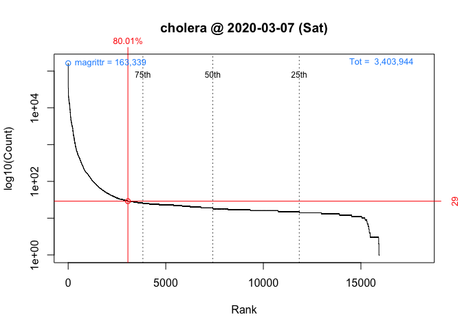
These graphs above, which are customized here to be on the same scale, plot the rank order of packages’ download counts (x-axis) against the logarithm of those counts (y-axis). It then highlights (in red) a package’s position in the distribution along with its rank percentile and download count. In the background, the 75th, 50th and 25th percentiles are plotted as dotted vertical lines. The package with the most downloads, ‘magrittr’ in both cases, is at top left (in blue). The total number of downloads is at the top right (in blue).
We compute the number of package downloads by simply counting log entries. While straightforward, this approach can run into problems. Putting aside the question of whether package dependencies should be counted, what I have in mind here is what I believe to be two types of “invalid” log entries. The first, a software artifact, stems from entries that are smaller, often orders of magnitude smaller, than a package’s actual binary or source file. The second, a behavioral artifact, emerges from efforts to download all of CRAN. In both cases, a reliance on nominal counts will give you an inflated sense of the degree of interest in your package. For those interested, an early but detailed analysis and discussion of both types of inflation is included as part of this R-hub blog post.
When looking at package download logs, the first thing you’ll notice are wrongly sized log entries. They come in two sizes. The “small” entries are approximately 500 bytes in size. The “medium” entries are variable in size: they fall somewhere between a “small” entry and a full download (i.e., “small” <= “medium” <= full download). “Small” entries manifest themselves as standalone entries, paired with a full download, or as part of a triplet along side a “medium” and a full download. “Medium” entries manifest themselves as either standalone entries or as part of a triplet.
The example below illustrates a triplet:
packageLog(date = "2020-07-01")[4:6, -(4:6)]
>               date     time    size package version country ip_id
> 3998633 2020-07-01 07:56:15   99622 cholera   0.7.0      US  4760
> 3999066 2020-07-01 07:56:15 4161948 cholera   0.7.0      US  4760
> 3999178 2020-07-01 07:56:15     536 cholera   0.7.0      US  4760
The “medium” entry is the first observation (99,622 bytes). The full download is the second entry (4,161,948 bytes). The “small” entry is the last observation (536 bytes). At a minimum, what makes a triplet a triplet (or a pair a pair) is that all members share system configuration (e.g. IP address, etc.) and have identical or adjacent time stamps.
To deal with the inflationary effect of “small” entries, I filter out observations smaller than 1,000 bytes (the smallest package on CRAN appears to be ‘source.gist’, which weighs in at 1,200 bytes). “Medium” entries are harder to handle. I remove them using either a triplet-specific filter or a filter that looks up a package’s actual size.
While wrongly sized entries are fairly easy to spot, seeing the effect of efforts to download all of CRAN require a change of perspective. While details and further evidence can be found in the R-hub blog post mentioned above, I’ll illustrate the problem with the following example:
packageLog(packages = "cholera", date = "2020-07-31")[8:14, -(4:6)]> date time size package version country ip_id
> 132509 2020-07-31 21:03:06 3797776 cholera 0.2.1 US 14
> 132106 2020-07-31 21:03:07 4285678 cholera 0.4.0 US 14
> 132347 2020-07-31 21:03:07 4109051 cholera 0.3.0 US 14
> 133198 2020-07-31 21:03:08 3766514 cholera 0.5.0 US 14
> 132630 2020-07-31 21:03:09 3764848 cholera 0.5.1 US 14
> 133078 2020-07-31 21:03:11 4275831 cholera 0.6.0 US 14
> 132644 2020-07-31 21:03:12 4284609 cholera 0.6.5 US 14Here, we see that seven different versions of the package were downloaded as a sequential bloc. A little digging shows that these seven versions represent all versions of ‘cholera’ available on that date:
packageHistory(package = "cholera")> Package Version Date Repository
> 1 cholera 0.2.1 2017-08-10 Archive
> 2 cholera 0.3.0 2018-01-26 Archive
> 3 cholera 0.4.0 2018-04-01 Archive
> 4 cholera 0.5.0 2018-07-16 Archive
> 5 cholera 0.5.1 2018-08-15 Archive
> 6 cholera 0.6.0 2019-03-08 Archive
> 7 cholera 0.6.5 2019-06-11 Archive
> 8 cholera 0.7.0 2019-08-28 CRANWhile there are “legitimate” reasons for downloading past versions (e.g., research, container-based software distribution, etc.), I’d argue that examples like the above are “fingerprints” of efforts to download CRAN. While this is not necessarily problematic, it does mean that when your package is downloaded as part of such efforts, that download is more a reflection of an interest in CRAN itself (a collection of packages) than of an interest in your package per se. And since one of the uses of counting package downloads is to assess interest in your package, it may be useful to exclude such entries.
To do so, I try to filter out these entries in two ways. The first identifies IP addresses that download “too many” packages and then filters out campaigns, large blocs of downloads that occur in (nearly) alphabetical order. The second looks for campaigns not associated with “greedy” IP addresses and filters out sequences of past versions downloaded in a narrowly defined time window.
To get an idea of how inflated your package’s download count may be,
use filteredDownloads(). Below are the results for
‘ggplot2’ for 15 September 2021.
filteredDownloads(package = "ggplot2", date = "2021-09-15")
>         date package downloads filtered.downloads inflation
> 1 2021-09-15 ggplot2    113842              58067     96.05
While there were 113,842 nominal downloads, applying all the filters reduced that number to 57,951, an inflation of 96%.
Note that the filters are computationally demanding. Excluding the time it takes to download the log file, the filters in the above example take approximate 75 seconds to run using parallelized code (currently only available on macOS and Unix) on a 3.1 GHz Dual-Core Intel Core i5 processor.
There are 5 filters. You can control them using the following arguments (listed in order of application):
ip.filter: removes campaigns of “greedy” IP
addresses.triplet.filter: reduces triplets to a single
observation.small.filter: removes entries smaller than 1,000
bytes.sequence.filter: removes blocs of past versions.size.filter: removes entries smaller than a package’s
binary or source file.These filters are off by default (e.g., ip.filter = FALSE). To apply them, set the argument for the filter you want to TRUE:
packageRank(package = "cholera", small.filter = TRUE)Alternatively, you can simply set
all.filters = TRUE.
packageRank(package = "cholera", all.filters = TRUE)Note that the all.filters = TRUE is contextual.
Depending on the function used, you’ll either get the CRAN-specific or
the package-specific set of filters. The former sets
ip.filter = TRUE and size.filter = TRUE; it
works independently of packages at the level of the entire log. The
latter sets triplet.filter = TRUE,
sequence.filter = TRUE and size.filter TRUE;
it relies on package specific information (e.g., size of source or
binary file).
Ideally, we’d like to use both sets. However, the package-specific
set is computationally expensive because they need to be applied
individually to all packages in the log, which can involve tens of
thousands of packages. While not unfeasible, currently this takes a long
time. For this reason, when all.filters = TRUE,
packageRank(), ipPackage(),
countryPackage(), countryDistribution() and
packageDistribution() use only CRAN specific filters while
packageLog(), packageCountry(), and
filteredDownloads() use both CRAN and package specific
filters.
Six other functions (some used above) may be of interest: 1)
packageDistribution() plots the location of your package in
the overall frequency distribution of package downloads; 2)
packageHistory() retrieves your package”s release history;
3) packageLog() extracts your package’s entries from the CRAN download counts log; 4)
filteredDownloads() computes an estimate of your package’s
download count inflation (computationally intensive!) and 5 & 6)
bioconductorDownloads() and bioconductorRank()
offer analogous but limited functionality to the two primary
functions.
While IP addresses are anonymized, packageCountry() and
countryPackage() make use of the fact that the logs provide
corresponding ISO country codes or top level domains (e.g., AT, JP, US).
Note that coverage extends to about 85% of observations (i.e.,
approximately 15% country codes are NA). Also, for what it’s worth,
there seems to be a a couple of typos for country codes: “A1” (A +
number one) and “A2” (A + number 2). According to RStudio’s documentation, this
coding was done using MaxMind’s free database, which no longer seems to
be available and may be a bit out of date.
fixDate_2012(), and
fixCranlogs()For those interested in directly using the RStudio download logs, this section describes some issues that may be of use.
The logs begin on 01 October 2012. Each day’s log is stored as a separate file with a name/URL that embeds the log’s date:
http://cran-logs.rstudio.com/2022/2022-01-01.csv.gzFor the logs of 2012, this convention was broken: 1) some logs are duplicated (same log, multiple names), 2) at least one is mislabeled, and 3) the logs from 13 October through 28 December are offset by +3 days (e.g., the file with the name/URL “2012-12-01” contains the log for “2012-11-28”). You can read the details here. Despite all this, only the last 3 logs of 2012 were lost.
For ‘packageRank’
functions that directly access logs via their filename/URL, like
packageRank() or packageLog(), fixDate_2012()
re-maps and resolves the issues above so that you’ll get the log you
expect.
The situation for packageRank::cranDownloads() is
different because that function is a modified wrapper of
cranlogs::cran_download(). On the plus side, it’s not
affected by the second and third problems. It’s my understanding that
this is because ‘cranlogs’ uses
the date in the log rather than log’s filename/URL. On the minus side,
it’s likely that functions and packages that depend on ‘cranlogs’ (e.g.,
‘adjustedcranlogs’,
‘dlstats’, packageRank::cranDownloads())
will be susceptible to the duplicate log problem.
Because ‘cranlogs’ relies on the date in the log and effectively ignores the log’s name/URL, it appears that ‘cranlogs’ can’t detect multiple instances of the same date’s log. While I found 3 logs with duplicate filename/URLs, my analysis turned up 5 additional instances of overcounting (including one of tripling).
I’ve patched this overcounting problem in packageRank::cranDownloads()
with fixCranlogs().
This function recomputes the data using the actual logs when any of the
eight problematic dates are requested. The details about the 8 days and
fixCranlogs() can be found here.
To avoid the bottleneck of downloading multiple log files,
packageRank() is currently limited to individual calendar
dates. To reduce the bottleneck of re-downloading logs, which can be
upwards of 50 MB, ‘packageRank’
makes use of memoization via the ‘memoise’
package.
Here’s relevant code:
fetchLog <- function(url) data.table::fread(url)

mfetchLog <- memoise::memoise(fetchLog)

if (RCurl::url.exists(url)) {
  cran_log <- mfetchLog(url)
}

# Note that data.table::fread() relies on R.utils::decompressFile().
This means that logs are intelligently cached; those that have already been downloaded in your current R session will not be downloaded again.
logInfo()The calendar date (e.g. “2021-01-01”) is the unit of observation for ‘packageRank’ functions. However, because you’re typically in today’s log file, time zone differences come into play.
Let’s say that it’s 09:01 on 01 January 2021 and you want to compute the rank percentile for ‘ergm’ for the last day of 2020. You might be tempted to use the following:
packageRank(packages = "ergm")However, depending on where you make this request, you may not get the data you expect. In Honolulu, USA, you will but in Sydney, Australia you won’t. The reason is that you’ve somehow forgotten a key piece of trivia: RStudio typically posts yesterday’s log around 17:00 UTC the following day.
The expression works in Honolulu because 09:01 HST on 01 January 2021 is 19:01 UTC 01 January 2021. So the log you want has been available for 2 hours. The expression fails in Sydney because 09:01 AEDT on 01 January 2021 is 31 December 2020 22:00 UTC. The log you want won’t actually be available for another 19 hours.
To make life a little easier, ‘packageRank’ does two things. First, when the log for the date you want is not available (due to time zone rather than server issues), you’ll just get the last available log. If you specified a date in the future, you’ll either get an error message or a warning that provides an estimate of when that log should be available.
Using the Sydney example and the expression above, you’d get the results for 30 December 2020:
packageRank(packages = "ergm")> date packages downloads rank percentile
> 1 2020-12-30 ergm 292 873 of 20,077 95.6If you had specified the date, you’d get an additional warning:
packageRank(packages = "ergm", date = "2021-01-01")> date packages downloads rank percentile
> 1 2020-12-30 ergm 292 873 of 20,077 95.6
Warning message:
2020-12-31 log arrives in appox. 19 hours at 02 Jan 04:00 AEDT. Using last available!Second, to help you check/remember when logs are posted in your
location, there’s logInfo(). The function returns the date
of the last available log and the date of “today’s” log. It then checks
to see if “today’s” log is posted on RStudio’s server and if today’s
results have been computed in ‘cranlogs’. If either or both fail, you’ll
see a range of contextual notes.
Keep in mind that 17:00 UTC is not a hard deadline. Barring server issues, the logs are usually posted before that time. I don’t know when the script starts but it seems to post closer to 17:00 UTC when a log has more entries than when it has fewer (i.e., weekdays v. weekends). Again barring software issues, the ‘cranlogs’ results are usually available shortly after 17:00 UTC.
Here’s what you’d see using the Honolulu example:
logInfo()$`Available log`
[1] "2021-01-01"
$`Today's log`
[1] "2020-12-31"
$`Today's log posted?`
[1] "Yes"
$`Today's results on 'cranlogs'?`
[1] "Yes"
$note
[1] "Everything OK."The functions uses your local time zone, which depends on R’s ability
to compute your local time and time zone (e.g., Sys.time()
and Sys.timezone()). My understanding is that there may be
operating system or platform specific issues that could undermine this
ability.
With R 4.0.3, the timeout value for internet connections became more explicit. Here are the relevant details from that release’s “New features”:
The default value for options("timeout") can be set from environment variable
R_DEFAULT_INTERNET_TIMEOUT, still defaulting to 60 (seconds) if that is not set
or invalid.
This change can affect functions that download logs. This is
especially true over slower internet connections or when you’re dealing
with large log files. To fix this, fetchCranLog() will, if
needed, temporarily set the timeout to 600 seconds.