paleopop is an extension to poems, a spatially-explicit, process-explicit, pattern-oriented framework for modeling population dynamics. This extension adds functionality for modeling large populations at generational time-steps over paleontological time-scales.
You can install the development version from GitHub with:
poems and paleopop are based on R6 class objects. R is primarily a functional programming language; if you want to simulate a population, you might use the lapply or replicate functions to repeat a generative function like rnorm. R6 creates an object-oriented programming language inside of R, so instead of using functions on other functions, in these packages we simulate populations using methods attached to objects. Think of R6 objects like machines, and methods like switches you can flip on the machines.
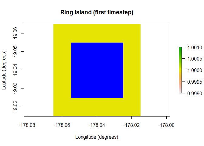
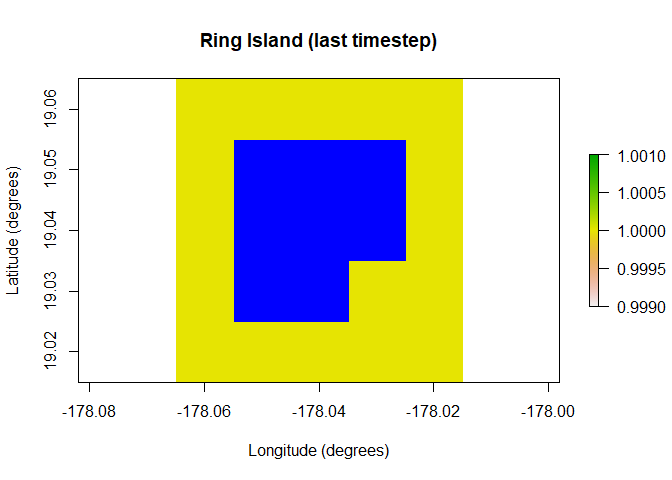
One of the major additions in paleopop is the PaleoRegion R6 class, which allows for regions that change over time due to ice sheets, sea level, bathymetry, and so on. The plots below show the temporal mask functionality of the PaleoRegion object. The temporal mask indicates cells that are occupiable at each time step with a 1 and unoccupiable cells with a NA. In this example, I use the temporal_mask_raster method to show how “Ring Island” changes at time step 10 due to a drop in sea level.
library(poems)
library(paleopop)
coordinates <- data.frame(x = rep(seq(-178.02, -178.06, -0.01), 5),
                          y = rep(seq(19.02, 19.06, 0.01), each = 5),
                          z = rep(1, 25))
template_raster <- raster::rasterFromXYZ(coordinates,
                                         crs = "+proj=longlat +datum=WGS84 +ellps=WGS84 +towgs84=0,0,0")
sealevel_raster <- template_raster
template_raster[][c(7:9, 12:14, 17:19)] <- NA # make Ring Island
sealevel_raster[][c(7:9, 12:14, 17:18)] <- NA
raster_stack <- raster::stack(x = append(replicate(9, template_raster), sealevel_raster))
region <- PaleoRegion$new(template_raster = raster_stack)
raster::plot(region$temporal_mask_raster()[[1]], main = "Ring Island (first timestep)",
             xlab = "Longitude (degrees)", ylab = "Latitude (degrees)",
             colNA = "blue")
raster::plot(region$temporal_mask_raster()[[10]], main = "Ring Island (last timestep)",
             xlab = "Longitude (degrees)", ylab = "Latitude (degrees)",
             colNA = "blue")
paleopop also includes the PaleoPopModel class, which sets up the population model structure. Here I show a very minimalist setup of a model template using this class.
model_template <- PaleoPopModel$new(
  region = region, # makes the simulation spatially explicit
  time_steps = 10, # number of time steps to simulate
  years_per_step = 12, # years per generational time-step
  standard_deviation = 0.1, # SD of growth rate
  growth_rate_max = 0.6, # maximum growth rate
  harvest = F, # are the populations harvested?
  populations = 17, # total occupiable cells over time
  initial_abundance = seq(9000, 0, -1000), # initial pop. sizes
  transition_rate = 1.0, # transition rate between generations
  carrying_capacity = rep(1000, 17), # static carrying capacity
  dispersal = (!diag(nrow = 17, ncol = 17))*0.05, # dispersal rates
  density_dependence = "logistic", # type of density dependence
  dispersal_target_k = 10, # minimum carrying capacity to attract dispersers
  occupancy_threshold = 1, # lower than this # of pops. means extinction
  abundance_threshold = 10, # threshold for Allee effect
  results_selection = c("abundance") # what outputs do you want in results?
)
The paleopop_simulator function accepts a PaleoPopModel object or a named list as input to simulate populations over paleo time scales, and the PaleoPopResults class stores the outputs from the paleo population simulator.
results <- paleopop_simulator(model_template)
results # examine
#> $abundance
#>       [,1] [,2] [,3] [,4] [,5] [,6] [,7] [,8] [,9] [,10]
#>  [1,]   39   74  150  252  424  666  667  766  871   995
#>  [2,]  117  229  374  528  670  930  777  878  832   963
#>  [3,] 1345 1063  913  938 1006  846  764  967  801   765
#>  [4,]   27   63   99  171  315  531  825  905 1081   898
#>  [5,]  382  532  707  846  979  940 1065  931 1023   977
#>  [6,]  523  715  876 1062 1113 1092 1355 1377  922   684
#>  [7,]  739  906  872  916 1183 1164 1086 1047  918   972
#>  [8,] 1238 1230 1400 1011 1093 1209 1184 1208 1007   953
#>  [9,] 1178 1100  954  999  916  831  745  881  928  1049
#> [10,]    0    0    0    0    0    0    0    0    0     0
#> [11,]    0    0    0    0    0    0    0    0    0     0
#> [12,]    0    0    0    0    0    0    0    0    0     0
#> [13,]  450  615  682  811  852 1035  984  951 1042  1055
#> [14,]  174  258  377  603  779  889  934  978  974   942
#> [15,]  600  805  948  919  887  926 1043  867 1003   866
#> [16,] 1313  882 1015 1052 1020  964  925 1003 1008  1049
#> [17,]  904 1035  983 1154 1043  887  907 1043  969   940
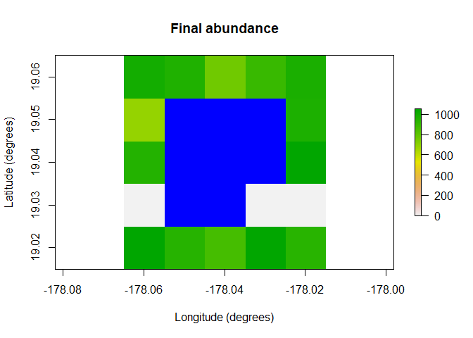
raster::plot(region$raster_from_values(results$abundance[,10]),
             main = "Final abundance", xlab = "Longitude (degrees)",
             ylab = "Latitude (degrees)", colNA = "blue")
A practical example of how to use paleopop, with more complex parameterization, can be found in the vignette.