This package implements an imputation approach to estimating path-specific effects (PSEs) in causal mediation analysis (Zhou and Yamamoto 2020). Estimation uncertainty is assessed using the nonparametric bootstrap.
You can install the released version of paths from CRAN with:
And the development version from GitHub with:
Given a binary treatment A, an outcome of interest Y, a set of pretreatment confounders X, and K causally ordered (possibly vector-valued) mediators M1, M2,…MK, the average total effect of the treatment on the outcome can be decomposed into K+1 PSEs that represent the causal paths A → M1 ⤳ Y, A → M2 ⤳ Y,… A → MK → Y, and A → Y, where the straight arrow → denotes a direct path and the squiggly arrow ⤳ represents a combination of all direct and indirect paths. These effects are nonparametrically identified under standard ignorability assumptions (Avin, Shpitser and Pearl 2005).
The paths function estimates these PSEs using an imputation approach, which requires the user to provide K+1 outcome models that characterize E[Y | X, A], E[Y | X, A, M1], …E[Y | X, A, MK], respectively. These outcome models can be objects returned by lm, glm, gbm::gbm, BART::pbart, or BART::wbart. Below is an example illustrating the use of paths to estimate the direct and indirect effects of ancestor victimization on descendants’ political attitudes. The original data come from Lupu and Peisakhin (2017).
library(paths)
library(gbm)

# K=3 causally ordered mediators
m1 <- c("trust_g1", "victim_g1", "fear_g1")
m2 <- c("trust_g2", "victim_g2", "fear_g2")
m3 <- c("trust_g3", "victim_g3", "fear_g3")
mediators <- list(m1, m2, m3)

# outcome model formulas
formula_m0 <- annex ~ kulak + prosoviet_pre + religiosity_pre + land_pre +
  orchard_pre + animals_pre + carriage_pre + otherprop_pre + violence
formula_m1 <- update(formula_m0,    ~ . + trust_g1 + victim_g1 + fear_g1)
formula_m2 <- update(formula_m1,    ~ . + trust_g2 + victim_g2 + fear_g2)
formula_m3 <- update(formula_m2,    ~ . + trust_g3 + victim_g3 + fear_g3)

# outcome models
gbm_m0 <- gbm(formula_m0, data = tatar, distribution = "bernoulli",
              interaction.depth = 3)
gbm_m1 <- gbm(formula_m1, data = tatar, distribution = "bernoulli",
              interaction.depth = 3)
gbm_m2 <- gbm(formula_m2, data = tatar, distribution = "bernoulli",
              interaction.depth = 3)
gbm_m3 <- gbm(formula_m3, data = tatar, distribution = "bernoulli",
              interaction.depth = 3)
gbm_ymodels <- list(gbm_m0, gbm_m1, gbm_m2, gbm_m3)

# causal paths analysis using gbm
tatar_paths <- paths(a = "violence", y = "annex", m = mediators,
  gbm_ymodels, data = tatar, nboot = 250)

# summarize results
summary(tatar_paths)
#>
#> Causal Paths Analysis
#>
#> Call: paths(a = "violence", y = "annex", m = mediators, models = gbm_ymodels,
#>     data = tatar, nboot = 250)
#>
#> Treatment: violence
#> Outcome: annex
#>
#> Outcome model: annex ~ kulak + prosoviet_pre + religiosity_pre + land_pre +
#>     orchard_pre + animals_pre + carriage_pre + otherprop_pre +
#>     violence
#> <environment: 0x000000001fd2b5c8>
#>
#> Mediator 1 :  trust_g1 + victim_g1 + fear_g1
#> Mediator 2 :  trust_g2 + victim_g2 + fear_g2
#> Mediator 3 :  trust_g3 + victim_g3 + fear_g3
#>
#> Causal Paths Estimates:
#>
#> Pure Imputation Estimator:
#> Type 1 Decomposition:
#>                               Estimate Std. Err. 95% CI Lower 95% CI Upper
#> Direct Effect: A -> Y            0.007     0.038       -0.089        0.054
#> Indirect Effect: A -> M3 -> Y   -0.037     0.024       -0.068        0.020
#> Indirect Effect: A -> M2 ~> Y   -0.025     0.024       -0.073        0.022
#> Indirect Effect: A -> M1 ~> Y   -0.114     0.025       -0.163       -0.068
#> Total Effect: A ~> Y            -0.169     0.051       -0.277       -0.077
#>                               P-value
#> Direct Effect: A -> Y           0.960
#> Indirect Effect: A -> M3 -> Y   0.384
#> Indirect Effect: A -> M2 ~> Y   0.328
#> Indirect Effect: A -> M1 ~> Y  <2e-16 ***
#> Total Effect: A ~> Y           <2e-16 ***
#> ---
#> Signif. codes:  0 '***' 0.001 '**' 0.01 '*' 0.05 '.' 0.1 ' ' 1
#>
#> Type 2 Decomposition:
#>                               Estimate Std. Err. 95% CI Lower 95% CI Upper
#> Direct Effect: A -> Y           -0.030     0.035       -0.119        0.014
#> Indirect Effect: A -> M3 -> Y   -0.029     0.023       -0.070        0.018
#> Indirect Effect: A -> M2 ~> Y   -0.018     0.024       -0.065        0.026
#> Indirect Effect: A -> M1 ~> Y   -0.093     0.030       -0.152       -0.034
#> Total Effect: A ~> Y            -0.169     0.051       -0.277       -0.077
#>                               P-value
#> Direct Effect: A -> Y            0.20
#> Indirect Effect: A -> M3 -> Y    0.36
#> Indirect Effect: A -> M2 ~> Y    0.52
#> Indirect Effect: A -> M1 ~> Y  <2e-16 ***
#> Total Effect: A ~> Y           <2e-16 ***
#> ---
#> Signif. codes:  0 '***' 0.001 '**' 0.01 '*' 0.05 '.' 0.1 ' ' 1
#>
#>
#> Sample size: 427
#>
#> Number of bootstrap simulations: 250The same PSEs can be alternatively estimated using an imputation-based weighting estimator detailed in Zhou and Yamamoto (2020). To implement this estimator, the user needs to additionally supply a propensity score model for the treatment, which can be objects returned by glm, gbm::gbm. twang::ps, or BART::pbart.
# propensity score model via gbm
formula_ps <- violence ~ kulak + prosoviet_pre + religiosity_pre + land_pre +
  orchard_pre + animals_pre + carriage_pre + otherprop_pre
gbm_ps <- gbm(formula_ps, data = tatar, distribution = "bernoulli",
              interaction.depth = 3)

# causal paths analysis using both the pure imputation estimator and the imputation-based weighting estimator
tatar_paths2 <- paths(a = "violence", y = "annex", m = mediators,
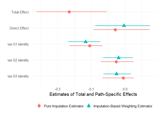
ps_model = gbm_ps, gbm_ymodels, data = tatar, nboot = 250)The plot.paths method can be used to visualize the total and path-specific causal effects estimated by paths.
plot(tatar_paths2, mediator_names = c("G1 identity", "G2 identity", "G3 identity"),
     estimator = "both")
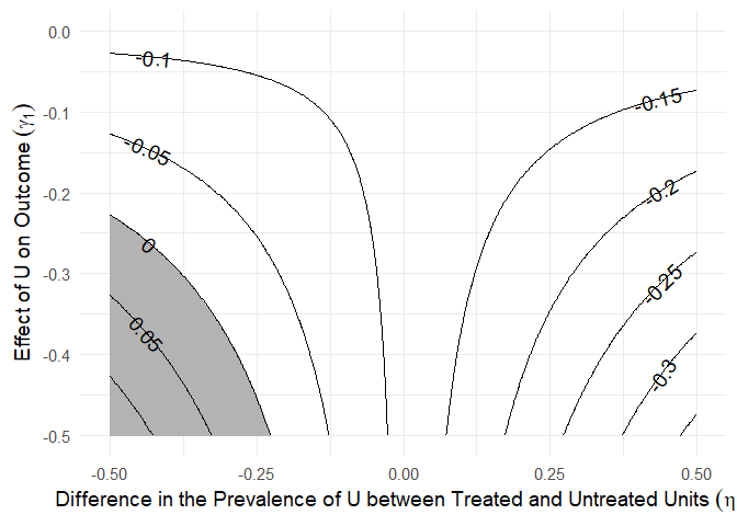
The sens() function implements a set of bias formulas detailed in Zhou and Yamamoto (2020) for assessing the sensitivity of estimated PSEs to an unobserved confounder U of a mediator-outcome relationship. The user provides a fitted paths object, the mediator whose relationship with the outcome is potentially confounded, the estimand whose sensitivity to unobserved confounding is being investigated, type of estimator, type of decomposition, and possible values of the sensitivity parameters γ and η.
The object returned by the sens() function is a list containing (a) the original estimate of the corresponding PSE, and (b) a data frame where each row represents a potential combination of γ and η, the corresponding bias, bias-adjusted estimate, and an indicator for whether the bias-adjusted estimate is of the opposite sign to the original estimate.
The plot.sens() function visualizes the sensitivity analysis by showing contours of bias-adjusted estimates under different values of γ and η.
# sensitivity analysis for the path-specific effect via M1
sens_paths <- sens(tatar_paths, confounded = "M1", estimand = "via M1",
  gamma_values = - seq(0, 0.5, 0.002), eta_values = seq(-0.5, 0.5, 0.002))

plot(sens_paths)
In experimental data where treatment is randomly assigned, the pure imputation estimator and the imputation-based weighting estimator are equivalent, so that a propensity score model for the treatment is not needed. In addition, because the treatment-outcome relationship is not confounded, the pretreatment covariates X can be omitted from the baseline model. Below is an example illustrating the use of paths to estimate the direct and indirect effects of issue framing on citizens’ support for welfare reform (Slothuus 2008). In this example, the treatment (issue framing) has been randomly assigned via a survey experiment so the baseline outcome model can be a simple linear regression of Y on A.
# variable names
x <- c("gender1", "educ1", "polint1", "ideo1", "know1", "value1")
a <- "ttt"
m1 <- c("W1", "W2")
m2 <- c("M1","M2","M3","M4","M5")
y <- "Y"
m <- list(m1, m2)

# formulas
form_m0 <- as.formula(paste0(y, "~", a))
form_m1 <- as.formula(paste0(y, "~", paste0(c(x, a, m1), collapse = "+")))
form_m2 <- as.formula(paste0(y, "~", paste0(c(x, a, m1, m2), collapse = "+")))

# baseline model for overall treatment effect
lm_m0 <- lm(form_m0, data = welfare)

# GBM outcome models
gbm_m1 <- gbm(form_m1, data = welfare, distribution = "gaussian",
              interaction.depth = 3)
gbm_m2 <- gbm(form_m2, data = welfare, distribution = "gaussian",
              interaction.depth = 3)
gbm_ymodels <- list(lm_m0, gbm_m1, gbm_m2)

# causal paths analysis
welfare_paths <- paths(a, y, m, models = gbm_ymodels,
                     data = welfare, nboot = 250)