

![]()
phylocomr gives you access to the Phylocom C library, licensed under BSD 2-clause
ecovolve/ph_ecovolve - interface to ecovolve executable, and a higher level interfacephylomatic/ph_phylomatic - interface to phylomatic executable, and a higher level interfacephylocom - interface to phylocom executableph_aot - higher level interface to aotph_bladj - higher level interface to bladjph_comdist/ph_comdistnt - higher level interface to comdistph_comstruct - higher level interface to comstructph_comtrait - higher level interface to comtraitph_pd - higher level interface to Faith’s phylogenetic diversityAs a convienence you can pass ages, sample and trait data.frame’s, and phylogenies as strings, to phylocomr functions. However, phylocomr has to write these data.frame’s/strings to disk (your computer’s file system) to be able to run the Phylocom code on them. Internally, phylocomr is writing to a temporary file to run Phylocom code, and then the file is removed.
In addition, you can pass in files instead of data.frame’s/strings. These are not themselves used. Instead, we read and write those files to temporary files. We do this for two reasons. First, Phylocom expects the files its using to be in the same directory, so if we control the file paths that becomes easier. Second, Phylocom is case sensitive, so we simply standardize all taxon names by lower casing all of them. We do this case manipulation on the temporary files so that your original data files are not modified.
Stable version:
Development version:
taxa_file <- system.file("examples/taxa", package = "phylocomr")
phylo_file <- system.file("examples/phylo", package = "phylocomr")
(taxa_str <- readLines(taxa_file))
#> [1] "campanulaceae/lobelia/lobelia_conferta"
#> [2] "cyperaceae/mapania/mapania_africana"
#> [3] "amaryllidaceae/narcissus/narcissus_cuatrecasasii"#> [1] "(((((eliea_articulata,homalanthus_populneus)malpighiales,rosa_willmottiae),((macrocentrum_neblinae,qualea_clavata),hibiscus_pohlii)malvids),(((lobelia_conferta,((millotia_depauperata,(layia_chrysanthemoides,layia_pentachaeta)layia),senecio_flanaganii)asteraceae)asterales,schwenkia_americana),tapinanthus_buntingii)),(narcissus_cuatrecasasii,mapania_africana))poales_to_asterales;"#> [1] "(lobelia_conferta:5.000000,(mapania_africana:1.000000,narcissus_cuatrecasasii:1.000000):1.000000)poales_to_asterales:1.000000;\n"
#> attr(,"taxa_file")
#> [1] "/var/folders/fc/n7g_vrvn0sx_st0p8lxb3ts40000gn/T//RtmpLApP50/taxa_c8d610d7337b"
#> attr(,"phylo_file")
#> [1] "/var/folders/fc/n7g_vrvn0sx_st0p8lxb3ts40000gn/T//RtmpLApP50/phylo_c8d62074d8e0"use various different references trees
library(brranching)
library(ape)

r2 <- ape::read.tree(text=brranching::phylomatic_trees[['R20120829']])
smith2011 <- ape::read.tree(text=brranching::phylomatic_trees[['smith2011']])
zanne2014 <- ape::read.tree(text=brranching::phylomatic_trees[['zanne2014']])

# R20120829 tree
taxa_str <- c(
  "asteraceae/bidens/bidens_alba",
  "asteraceae/cirsium/cirsium_arvense",
  "fabaceae/lupinus/lupinus_albus"
)
ph_phylomatic(taxa = taxa_str, phylo = r2)
#> [1] "(((bidens_alba:13.000000,cirsium_arvense:13.000000):19.000000,lupinus_albus:27.000000):12.000000)euphyllophyte:1.000000;\n"
#> attr(,"taxa_file")
#> [1] "/var/folders/fc/n7g_vrvn0sx_st0p8lxb3ts40000gn/T//RtmpLApP50/taxa_c8d656a7d848"
#> attr(,"phylo_file")
#> [1] "/var/folders/fc/n7g_vrvn0sx_st0p8lxb3ts40000gn/T//RtmpLApP50/phylo_c8d625688b6a"# zanne2014 tree
taxa_str <- c(
"zamiaceae/dioon/dioon_edule",
"zamiaceae/encephalartos/encephalartos_dyerianus",
"piperaceae/piper/piper_arboricola"
)
ph_phylomatic(taxa = taxa_str, phylo = zanne2014)#> [1] "(((dioon_edule:121.744843,encephalartos_dyerianus:121.744850)zamiaceae:230.489838,piper_arboricola:352.234711)spermatophyta:88.058670):0.000000;\n"
#> attr(,"taxa_file")
#> [1] "/var/folders/fc/n7g_vrvn0sx_st0p8lxb3ts40000gn/T//RtmpLApP50/taxa_c8d67298ef55"
#> attr(,"phylo_file")
#> [1] "/var/folders/fc/n7g_vrvn0sx_st0p8lxb3ts40000gn/T//RtmpLApP50/phylo_c8d61688f03a"# zanne2014 subtree
zanne2014_subtr <- ape::extract.clade(zanne2014, node='Loganiaceae')
zanne_subtree_file <- tempfile(fileext = ".txt")
ape::write.tree(zanne2014_subtr, file = zanne_subtree_file)
taxa_str <- c(
"loganiaceae/neuburgia/neuburgia_corynocarpum",
"loganiaceae/geniostoma/geniostoma_borbonicum",
"loganiaceae/strychnos/strychnos_darienensis"
)
ph_phylomatic(taxa = taxa_str, phylo = zanne2014_subtr)#> [1] "((neuburgia_corynocarpum:32.807743,(geniostoma_borbonicum:32.036335,strychnos_darienensis:32.036335):0.771406):1.635496)loganiaceae:0.000000;\n"
#> attr(,"taxa_file")
#> [1] "/var/folders/fc/n7g_vrvn0sx_st0p8lxb3ts40000gn/T//RtmpLApP50/taxa_c8d630ca1ff3"
#> attr(,"phylo_file")
#> [1] "/var/folders/fc/n7g_vrvn0sx_st0p8lxb3ts40000gn/T//RtmpLApP50/phylo_c8d625f7a38b"#> [1] "((neuburgia_corynocarpum:32.807743,(geniostoma_borbonicum:32.036335,strychnos_darienensis:32.036335):0.771406):1.635496)loganiaceae:0.000000;\n"
#> attr(,"taxa_file")
#> [1] "/var/folders/fc/n7g_vrvn0sx_st0p8lxb3ts40000gn/T//RtmpLApP50/taxa_c8d625120e26"
#> attr(,"phylo_file")
#> [1] "/var/folders/fc/n7g_vrvn0sx_st0p8lxb3ts40000gn/T//RtmpLApP50/phylo_c8d6445ef3cd"traits_file <- system.file("examples/traits_aot", package = "phylocomr")
phylo_file <- system.file("examples/phylo_aot", package = "phylocomr")
traitsdf_file <- system.file("examples/traits_aot_df", package = "phylocomr")
traits <- read.table(text = readLines(traitsdf_file), header = TRUE,
stringsAsFactors = FALSE)
phylo_str <- readLines(phylo_file)
ph_aot(traits = traits, phylo = phylo_str)#> $trait_conservatism
#> # A tibble: 124 x 28
#> trait trait.name node name age ntaxa n.nodes tip.mn tmn.ranklow
#> <int> <chr> <int> <chr> <dbl> <int> <int> <dbl> <int>
#> 1 1 traitA 0 a 5 32 2 1.75 1000
#> 2 1 traitA 1 b 4 16 2 1.75 638
#> 3 1 traitA 2 c 3 8 2 1.75 645
#> 4 1 traitA 3 d 2 4 2 1.5 238
#> 5 1 traitA 4 e 1 2 2 1 51
#> 6 1 traitA 7 f 1 2 2 2 1000
#> 7 1 traitA 10 g 2 4 2 2 1000
#> 8 1 traitA 11 h 1 2 2 2 1000
#> 9 1 traitA 14 i 1 2 2 2 1000
#> 10 1 traitA 17 j 3 8 2 1.75 663
#> # … with 114 more rows, and 19 more variables: tmn.rankhi <int>, tip.sd <dbl>,
#> # tsd.ranklow <int>, tsd.rankhi <int>, node.mn <dbl>, nmn.ranklow <int>,
#> # nmn.rankhi <int>, nod.sd <dbl>, nsd.ranklow <int>, nsd.rankhi <int>,
#> # sstipsroot <dbl>, sstips <dbl>, percvaramongnodes <dbl>,
#> # percvaratnode <dbl>, contributionindex <dbl>, sstipvnoderoot <dbl>,
#> # sstipvnode <dbl>, ssamongnodes <dbl>, sswithinnodes <dbl>
#>
#> $independent_contrasts
#> # A tibble: 31 x 17
#> node name age n.nodes contrast1 contrast2 contrast3 contrast4 contrastsd
#> <int> <chr> <dbl> <int> <dbl> <dbl> <dbl> <dbl> <dbl>
#> 1 0 a 5 2 0 0 0 0.254 1.97
#> 2 1 b 4 2 0 1.03 0 0.516 1.94
#> 3 2 c 3 2 0.267 0.535 0 0 1.87
#> 4 3 d 2 2 0.577 0 1.15 0 1.73
#> 5 4 e 1 2 0 0 0.707 0 1.41
#> 6 7 f 1 2 0 0 0.707 0 1.41
#> 7 10 g 2 2 0 0 1.15 0 1.73
#> 8 11 h 1 2 0 0 0.707 0 1.41
#> 9 14 i 1 2 0 0 0.707 0 1.41
#> 10 17 j 3 2 0.267 0.535 0 0 1.87
#> # … with 21 more rows, and 8 more variables: lowval1 <dbl>, hival1 <dbl>,
#> # lowval2 <dbl>, hival2 <dbl>, lowval3 <dbl>, hival3 <dbl>, lowval4 <dbl>,
#> # hival4 <dbl>
#>
#> $phylogenetic_signal
#> # A tibble: 4 x 5
#> trait ntaxa varcontr varcn.ranklow varcn.rankhi
#> <chr> <int> <dbl> <int> <int>
#> 1 traitA 32 0.054 1 1000
#> 2 traitB 32 0.109 1 1000
#> 3 traitC 32 0.622 67 934
#> 4 traitD 32 0.011 1 1000
#>
#> $ind_contrast_corr
#> # A tibble: 3 x 6
#> xtrait ytrait ntaxa picr npos ncont
#> <chr> <chr> <int> <dbl> <dbl> <int>
#> 1 traitA traitB 32 0.248 18.5 31
#> 2 traitA traitC 32 0.485 27.5 31
#> 3 traitA traitD 32 0 16.5 31ages_file <- system.file("examples/ages", package = "phylocomr")
phylo_file <- system.file("examples/phylo_bladj", package = "phylocomr")
ages_df <- data.frame(
a = c('malpighiales','salicaceae','fabaceae','rosales','oleaceae',
'gentianales','apocynaceae','rubiaceae'),
b = c(81,20,56,76,47,71,18,56)
)
phylo_str <- readLines(phylo_file)
(res <- ph_bladj(ages = ages_df, phylo = phylo_str))#> [1] "((((((lomatium_concinnum:20.250000,campanula_vandesii:20.250000):20.250000,(((veronica_candidissima:10.125000,penstemon_paniculatus:10.125000)plantaginaceae:10.125000,justicia_oblonga:20.250000):10.125000,marsdenia_gilgiana:30.375000):10.125000):10.125000,epacris_alba-compacta:50.625000)ericales_to_asterales:10.125000,((daphne_anhuiensis:20.250000,syzygium_cumini:20.250000)malvids:20.250000,ditaxis_clariana:40.500000):20.250000):10.125000,thalictrum_setulosum:70.875000)eudicots:10.125000,((dendrocalamus_giganteus:27.000000,guzmania_densiflora:27.000000)poales:27.000000,warczewiczella_digitata:54.000000):27.000000)malpighiales:1.000000;\n"
#> attr(,"ages_file")
#> [1] "/var/folders/fc/n7g_vrvn0sx_st0p8lxb3ts40000gn/T//RtmpLApP50/ages"
#> attr(,"phylo_file")
#> [1] "/var/folders/fc/n7g_vrvn0sx_st0p8lxb3ts40000gn/T//RtmpLApP50/phylo_c8d65b2958fd"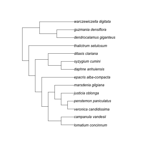
phylocomr in R doing citation(package = 'phylocomr')