The poems package provides a framework of interoperable R6 (Chang, 2020) classes for building ensembles of viable models via the pattern-oriented modeling (POM) approach (Grimm et al., 2005). The package includes classes for encapsulating and generating model parameters, and managing the POM workflow. The workflow includes:
By default, model validation and selection utilizes an approximate Bayesian computation (ABC) approach (Beaumont et al., 2002) using the abc package (Csillery et al., 2015). However, alternative user-defined functionality could be employed.
The package includes a spatially explicit demographic population model simulation engine, which incorporates default functionality for density dependence, correlated environmental stochasticity, stage-based transitions, and distance-based dispersal. The user may customize the simulator by defining functionality for trans-locations, harvesting, mortality, and other processes, as well as defining the sequence order for the simulator processes. The framework could also be adapted for use with other model simulators by utilizing its extendable (inheritable) base classes.
You can install the released version of poems from CRAN with:
And the development version from GitHub with:
The following simple example demonstrates how to run a single spatially explicit demographic population model using poems:
library(poems)
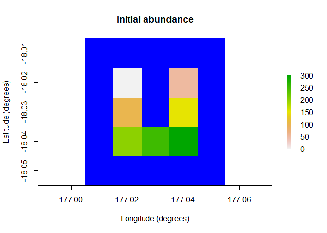
# Demonstration example region (U Island) and initial abundance
coordinates <- data.frame(x = rep(seq(177.01, 177.05, 0.01), 5),
y = rep(seq(-18.01, -18.05, -0.01), each = 5))
template_raster <- Region$new(coordinates = coordinates)$region_raster # full extent
template_raster[][-c(7, 9, 12, 14, 17:19)] <- NA # make U Island
region <- Region$new(template_raster = template_raster)
initial_abundance <- seq(0, 300, 50)
raster::plot(region$raster_from_values(initial_abundance),
main = "Initial abundance", xlab = "Longitude (degrees)",
ylab = "Latitude (degrees)", zlim = c(0, 300), colNA = "blue")
# Set population model
pop_model <- PopulationModel$new(
  region = region,
  time_steps = 5,
  populations = 7,
  initial_abundance = initial_abundance,
  stage_matrix = matrix(c(0, 2.5, # Leslie/Lefkovitch matrix
                          0.8, 0.5), nrow = 2, ncol = 2, byrow = TRUE),
  carrying_capacity = rep(200, 7),
  density_dependence = "logistic",
  dispersal = (!diag(nrow = 7, ncol = 7))*0.05,
  result_stages = c(1, 2))

# Run single simulation
results <- population_simulator(pop_model)
results # examine
#> $all
#> $all$abundance
#> [1] 1067 1107 1263 1327 1336
#>
#> $all$abundance_stages
#> $all$abundance_stages[[1]]
#> [1] 652 662 754 820 744
#>
#> $all$abundance_stages[[2]]
#> [1] 415 445 509 507 592
#>
#>
#>
#> $abundance
#>      [,1] [,2] [,3] [,4] [,5]
#> [1,]   52  124  154  177  193
#> [2,]  100  149  195  180  191
#> [3,]  129  153  159  179  173
#> [4,]  152  145  167  168  183
#> [5,]  219  169  202  204  216
#> [6,]  205  172  186  210  180
#> [7,]  210  195  200  209  200
#>
#> $abundance_stages
#> $abundance_stages[[1]]
#>      [,1] [,2] [,3] [,4] [,5]
#> [1,]   31   73   91  108  103
#> [2,]   67   76  118  110  119
#> [3,]   80   99  103  110  111
#> [4,]  100   74  108   93   99
#> [5,]  138   98  125  118  121
#> [6,]  121  113  106  145   84
#> [7,]  115  129  103  136  107
#>
#> $abundance_stages[[2]]
#>      [,1] [,2] [,3] [,4] [,5]
#> [1,]   21   51   63   69   90
#> [2,]   33   73   77   70   72
#> [3,]   49   54   56   69   62
#> [4,]   52   71   59   75   84
#> [5,]   81   71   77   86   95
#> [6,]   84   59   80   65   96
#> [7,]   95   66   97   73   93
raster::plot(region$raster_from_values(results$abundance[,5]),
             main = "Final abundance", xlab = "Longitude (degrees)",
             ylab = "Latitude (degrees)", zlim = c(0, 300), colNA = "blue")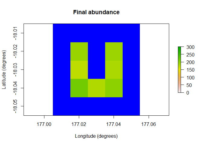
Further examples utilizing the POM workflow and more advanced features of poems can be found in the accompanying vignettes.
Beaumont, M. A., Zhang, W., & Balding, D. J. (2002). ‘Approximate Bayesian computation in population genetics’. Genetics, vol. 162, no. 4, pp, 2025–2035.
Chang, W. (2020). ‘R6: Encapsulated Classes with Reference Semantics’. R package version 2.5.0. Retrieved from https://CRAN.R-project.org/package=R6
Csillery, K., Lemaire L., Francois O., & Blum M. (2015). ‘abc: Tools for Approximate Bayesian Computation (ABC)’. R package version 2.1. Retrieved from https://CRAN.R-project.org/package=abc
Grimm, V., Revilla, E., Berger, U., Jeltsch, F., Mooij, W. M., Railsback, S. F., Thulke, H. H., Weiner, J., Wiegand, T., DeAngelis, D. L., (2005). ‘Pattern-Oriented Modeling of Agent-Based Complex Systems: Lessons from Ecology’. Science vol. 310, no. 5750, pp. 987–991.
Iman R. L., Conover W. J. (1980). ‘Small sample sensitivity analysis techniques for computer models, with an application to risk assessment’. Commun Stat Theor Methods A9, pp. 1749–1842.