![]()
The goal of rdecision is to provide methods for
assessing health care interventions using cohort models (decision trees
and semi-Markov models) which can be constructed using only a few lines
of R code. Mechanisms are provided for associating an uncertainty
distribution with each source variable and for ensuring transparency of
the mathematical relationships between variables. The package
terminology follows Briggs et al “Decision Modelling for Health
Economic Evaluation”.1
You can install the released version of rdecision from CRAN with:
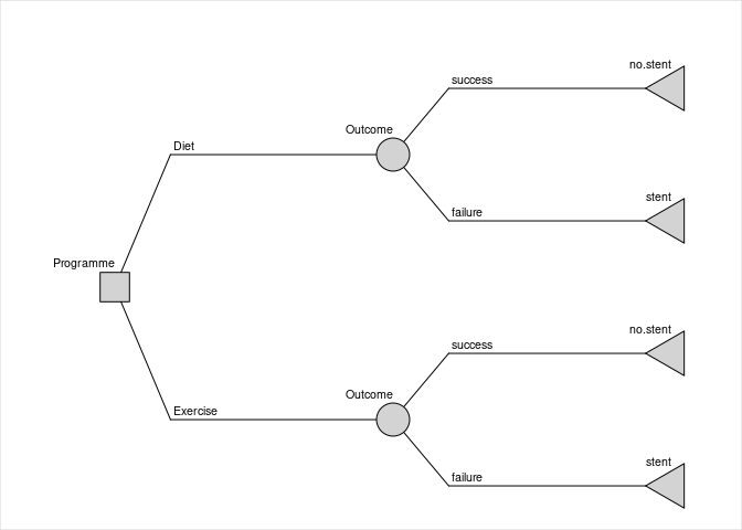
install.packages("rdecision")Consider the fictitious and idealized decision problem of choosing between providing two forms of lifestyle advice, offered to people with vascular disease, which reduce the risk of needing an interventional procedure. The model has a time horizon of 1 year. The cost to a healthcare provider of the interventional procedure (e.g. inserting a stent) is 5000 GBP; the cost of providing the current form of lifestyle advice, an appointment with a dietician (“diet”), is 50 GBP and the cost of providing an alternative form, attendance at an exercise programme (“exercise”), is 500 GBP. If the advice programme is successful, there is no need for an interventional procedure. In a small trial of the “diet” programme, 12 out of 68 patients (17.6%) avoided having a procedure, and in a separate small trial of the “exercise” programme 18 out of 58 patients (31.0%) avoided the procedure. It is assumed that the baseline characteristics in the two trials were comparable, that the model is from the perspective of the healthcare provider and that the utility is the same for all patients.
A decision tree can be constructed to estimate the uncertainty of the cost difference between the two types of advice programme, due to the finite sample sizes of each trial. The proportions of each advice programme being successful (i.e. avoiding intervention) are represented by model variables with uncertainties which follow Beta distributions. Probabilities of the failure of the programmes are calculated using expression model variables to ensure that the total probability associated with each chance node is one.
library("rdecision")
# probabilities of programme success & failure
p.diet <- BetaModVar$new("P(diet)", "", alpha=12, beta=68-12)
p.exercise <- BetaModVar$new("P(exercise)", "", alpha=18, beta=58-18)
q.diet <- ExprModVar$new("1-P(diet)", "", rlang::quo(1-p.diet))
q.exercise <- ExprModVar$new("1-P(exercise)", "", rlang::quo(1-p.exercise))
# costs
c.diet <- 50
c.exercise <- ConstModVar$new("Cost of exercise programme", "GBP", 500)
c.stent <- 5000
The decision tree is constructed from nodes and edges as follows:
t.ds <- LeafNode$new("no stent")
t.df <- LeafNode$new("stent")
t.es <- LeafNode$new("no stent")
t.ef <- LeafNode$new("stent")
c.d <- ChanceNode$new("Outcome")
c.e <- ChanceNode$new("Outcome")
d <- DecisionNode$new("Programme")

e.d <- Action$new(d, c.d, cost=c.diet, label = "Diet")
e.e <- Action$new(d, c.e, cost=c.exercise, label = "Exercise")
e.ds <- Reaction$new(c.d, t.ds, p=p.diet, cost = 0, label = "success")
e.df <- Reaction$new(c.d, t.df, p=q.diet, cost=c.stent, label="failure")
e.es <- Reaction$new(c.e, t.es, p=p.exercise, cost=0, label="success")
e.ef <- Reaction$new(c.e, t.ef, p=q.exercise, cost=c.stent, label="failure")

DT <- DecisionTree$new(
  V = list(d, c.d, c.e, t.ds, t.df, t.es, t.ef),
  E = list(e.d, e.e, e.ds, e.df, e.es, e.ef)
)
The expected per-patient net cost of each option is obtained by
evaluating the tree with expected values of all variables using
DT$evaluate() and threshold values with
DT$threshold(). Examination of the results of evaluation
shows that the expected per-patient net cost of the diet advice
programme is 4167.65 GBP and the per-patient net cost of the exercise
programme is 3948.28 GBP, a point estimate saving of 219.37 GBP per
patient if the exercise advice programme is adopted. By univariate
threshold analysis, the exercise program will be cost saving when its
cost of delivery is less than 719.73 GBP or when its success rate is
greater than 26.6%.
The confidence interval of the cost saving is estimated by repeated
evaluation of the tree, each time sampling from the uncertainty
distribution of the two probabilities using, for example,
DT$evaluate(setvars="random", N=1000) and inspecting the
resulting data frame. From 1000 runs, the 95% confidence interval of the
per patient cost saving is -473.76 GBP to 909.83 GBP, with 73.9% being
cost saving, and it can be concluded that more evidence is required to
be confident that the exercise programme is cost saving.
Sonnenberg and Beck2 introduced an illustrative example of
a semi-Markov process with three states: “Well”, “Disabled” and “Dead”
and one transition between each state, each with a per-cycle
probability. In rdecision such a model is constructed as
follows. Note that transitions from a state to itself must be specified
if allowed, otherwise the state would be a temporary state.
# create states
s.well <- MarkovState$new(name="Well", utility=1)
s.disabled <- MarkovState$new(name="Disabled",utility=0.7)
s.dead <- MarkovState$new(name="Dead",utility=0)
# create transitions, leaving rates undefined
E <- list(
  Transition$new(s.well, s.well),
  Transition$new(s.dead, s.dead),
  Transition$new(s.disabled, s.disabled),
  Transition$new(s.well, s.disabled),
  Transition$new(s.well, s.dead),
  Transition$new(s.disabled, s.dead)
)
# create the model
M <- SemiMarkovModel$new(V = list(s.well, s.disabled, s.dead), E)
# create transition probability matrix
snames <- c("Well","Disabled","Dead")
Pt <- matrix(
  data = c(0.6, 0.2, 0.2, 0, 0.6, 0.4, 0, 0, 1),
  nrow = 3, byrow = TRUE,
  dimnames = list(source=snames, target=snames)
)
# set the transition rates from per-cycle probabilities
M$set_probabilities(Pt)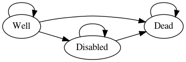
With a starting population of 10,000, the model can be run for 25
years as follows. The output of the cycles function is the
Markov trace, shown below, which replicates Table 2.2
# set the starting populations
M$reset(c(Well=10000, Disabled=0, Dead=0))
# cycle
MT <- M$cycles(25, hcc.pop=FALSE, hcc.cost=FALSE)| Years | Well | Disabled | Dead | Cumulative Utility |
|---|---|---|---|---|
| 0 | 10000 | 0 | 0 | 0 |
| 1 | 6000 | 2000 | 2000 | 0.74 |
| 2 | 3600 | 2400 | 4000 | 1.268 |
| 3 | 2160 | 2160 | 5680 | 1.635 |
| 23 | 0 | 1 | 9999 | 2.375 |
| 24 | 0 | 0 | 10000 | 2.375 |
| 25 | 0 | 0 | 10000 | 2.375 |
In addition to using base R,3 redecision
relies heavily on the R6 implementation of
classes4 and the rlang package for error
handling and non-standard evaluation used in expression model
variables.5 Building the package vignettes and documentation
relies on the testthat package,6 the
devtools package7 and
rmarkdown.10
Underpinning graph theory is based on terminology, definitions and algorithms from Gross et al,11 the Wikipedia glossary12 and links therein. Topological sorting of graphs is based on Kahn’s algorithm.13 Some of the terminology for decision trees was based on the work of Kaminski et al14 and an efficient tree drawing algorithm was based on the work of Walker.15 In semi-Markov models, representations are exported in the DOT language.16
Terminology for decision trees and Markov models in health economic evaluation was based on the book by Briggs et al1 and the output format and terminology follows ISPOR recommendations.18
Citations for examples used in vignettes are given in applicable vignette files.