![]()
“From R to your manuscript”
report’s primary goal is to bridge the gap between R’s output and the formatted results contained in your manuscript. It automatically produces reports of models and dataframes according to best practices guidelines (e.g., APA’s style), ensuring standardization and quality in results reporting.
library(report)

model <- lm(Sepal.Length ~ Species, data = iris)
report(model)
# We fitted a linear model (estimated using OLS) to predict Sepal.Length with Species (formula: Sepal.Length ~ Species). The model explains a statistically significant and substantial proportion of variance (R2 = 0.62, F(2, 147) = 119.26, p < .001, adj. R2 = 0.61). The model's intercept, corresponding to Species = setosa, is at 5.01 (95% CI [4.86, 5.15], t(147) = 68.76, p < .001). Within this model:
#
#   - The effect of Species [versicolor] is statistically significant and positive (beta = 0.93, 95% CI [0.73, 1.13], t(147) = 9.03, p < .001; Std. beta = 1.12, 95% CI [0.88, 1.37])
#   - The effect of Species [virginica] is statistically significant and positive (beta = 1.58, 95% CI [1.38, 1.79], t(147) = 15.37, p < .001; Std. beta = 1.91, 95% CI [1.66, 2.16])
#
# Standardized parameters were obtained by fitting the model on a standardized version of the dataset. 95% Confidence Intervals (CIs) and p-values were computed using the Wald approximation.![]()
![]()
![]()
The package documentation can be found here. Check-out these tutorials:
report is a young package in need of affection. You can easily be a part of the developing community of this open-source software and improve science! Don’t be shy, try to code and submit a pull request (See the contributing guide). Even if it’s not perfect, we will help you make it great!
The package is available on CRAN and can be downloaded by running:
If you would instead like to experiment with the development version, you can download it from GitHub:
install.packages("remotes")
remotes::install_github("easystats/report") # You only need to do that once
Load the package every time you start R

The report package works in a two step fashion. First, you create a report object with the report() function. Then, this report object can be displayed either textually (the default output) or as a table, using as.data.frame(). Moreover, you can also access a more digest and compact version of the report using summary() on the report object.
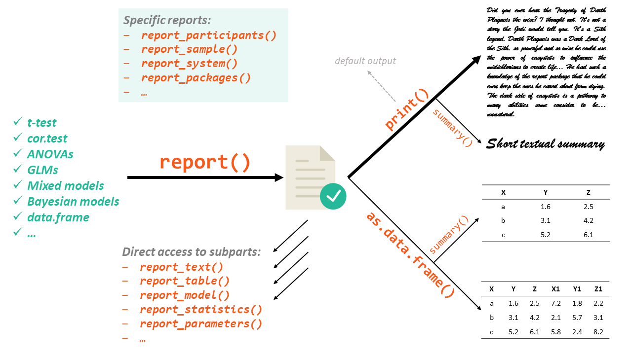
The report() function works on a variety of models, as well as other objects such as dataframes:
# The data contains 150 observations of the following 5 variables:
#   - Sepal.Length: n = 150, Mean = 5.84, SD = 0.83, Median = 5.80, MAD = 1.04,
# range: [4.30, 7.90], Skewness = 0.31, Kurtosis = -0.55, 0% missing
#   - Sepal.Width: n = 150, Mean = 3.06, SD = 0.44, Median = 3.00, MAD = 0.44,
# range: [2, 4.40], Skewness = 0.32, Kurtosis = 0.23, 0% missing
#   - Petal.Length: n = 150, Mean = 3.76, SD = 1.77, Median = 4.35, MAD = 1.85,
# range: [1, 6.90], Skewness = -0.27, Kurtosis = -1.40, 0% missing
#   - Petal.Width: n = 150, Mean = 1.20, SD = 0.76, Median = 1.30, MAD = 1.04,
# range: [0.10, 2.50], Skewness = -0.10, Kurtosis = -1.34, 0% missing
#   - Species: 3 levels, namely setosa (n = 50, 33.33%), versicolor (n = 50,
# 33.33%) and virginica (n = 50, 33.33%)
These reports nicely work within the tidyverse workflow:
# The data contains 150 observations, grouped by Species, of the following 3
# variables:
#
# - setosa (n = 50):
#   - Petal.Length: Mean = 1.46, SD = 0.17, range: [1, 1.90]
#   - Petal.Width: Mean = 0.25, SD = 0.11, range: [0.10, 0.60]
#
# - versicolor (n = 50):
#   - Petal.Length: Mean = 4.26, SD = 0.47, range: [3, 5.10]
#   - Petal.Width: Mean = 1.33, SD = 0.20, range: [1, 1.80]
#
# - virginica (n = 50):
#   - Petal.Length: Mean = 5.55, SD = 0.55, range: [4.50, 6.90]
# - Petal.Width: Mean = 2.03, SD = 0.27, range: [1.40, 2.50]Reports can be used to automatically format tests like t-tests or correlations.
# Effect sizes were labelled following Cohen's (1988) recommendations.
#
# The Welch Two Sample t-test testing the difference of mtcars$mpg by mtcars$am
# (mean in group 0 = 17.15, mean in group 1 = 24.39) suggests that the effect is
# negative, statistically significant, and large (difference = -7.24, 95% CI
# [-11.28, -3.21], t(18.33) = -3.77, p = 0.001; Cohen's d = -1.41, 95% CI [-2.26,
# -0.53])
As mentioned, you can also create tables with the as.data.frame() functions, like for example with this correlation test:
cor.test(iris$Sepal.Length, iris$Sepal.Width) %>%
  report() %>%
  as.data.frame()
# Error in abs(r): non-numeric argument to mathematical functionThis works great with ANOVAs, as it includes effect sizes and their interpretation.
# The ANOVA (formula: Sepal.Length ~ Species) suggests that:
#
#   - The main effect of Species is statistically significant and large (F(2, 147)
# = 119.26, p < .001; Eta2 = 0.62, 95% CI [0.54, 1.00])
#
# Effect sizes were labelled following Field's (2013) recommendations.Reports are also compatible with GLMs, such as this logistic regression:
# We fitted a logistic model (estimated using ML) to predict vs with mpg and drat
# (formula: vs ~ mpg * drat). The model's explanatory power is substantial
# (Tjur's R2 = 0.51). The model's intercept, corresponding to mpg = 0 and drat =
# 0, is at -33.43 (95% CI [-77.90, 3.25], p = 0.083). Within this model:
#
#   - The effect of mpg is statistically non-significant and positive (beta = 1.79,
# 95% CI [-0.10, 4.05], p = 0.066; Std. beta = 3.63, 95% CI [1.36, 7.50])
#   - The effect of drat is statistically non-significant and positive (beta =
# 5.96, 95% CI [-3.75, 16.26], p = 0.205; Std. beta = -0.36, 95% CI [-1.96,
# 0.98])
#   - The interaction effect of drat on mpg is statistically non-significant and
# negative (beta = -0.33, 95% CI [-0.83, 0.15], p = 0.141; Std. beta = -1.07, 95%
# CI [-2.66, 0.48])
#
#  Standardized parameters were obtained by fitting the model on a standardized
# version of the dataset. 95% Confidence Intervals (CIs) and p-values were
# computed using
Mixed models (coming from example from the lme4 package), which popularity and usage is exploding, can also be reported as it should:
library(lme4)

model <- lme4::lmer(Sepal.Length ~ Petal.Length + (1 | Species), data = iris)

report(model)
# We fitted a linear mixed model (estimated using REML and nloptwrap optimizer)
# to predict Sepal.Length with Petal.Length (formula: Sepal.Length ~
# Petal.Length). The model included Species as random effect (formula: ~1 |
# Species). The model's total explanatory power is substantial (conditional R2 =
# 0.97) and the part related to the fixed effects alone (marginal R2) is of 0.66.
# The model's intercept, corresponding to Petal.Length = 0, is at 2.50 (95% CI
# [1.19, 3.82], t(146) = 3.75, p < .001). Within this model:
#
# - The effect of Petal Length is statistically significant and positive (beta =
# 0.89, 95% CI [0.76, 1.01], t(146) = 13.93, p < .001; Std. beta = 1.89, 95% CI
# [1.63, 2.16])
#
# Standardized parameters were obtained by fitting the model on a standardized
# version of the dataset. 95% Confidence Intervals (CIs) and p-values were
# computed usingBayesian models can also be reported using the new SEXIT framework, that combines clarity, precision and usefulness.
# We fitted a Bayesian linear model (estimated using MCMC sampling with 4 chains
# of 1000 iterations and a warmup of 500) to predict mpg with qsec and wt
# (formula: mpg ~ qsec + wt). Priors over parameters were set as normal (mean =
# 0.00, SD = 8.43) and normal (mean = 0.00, SD = 15.40) distributions. The
# model's explanatory power is substantial (R2 = 0.81, 95% CI [0.69, 0.89], adj.
# R2 = 0.79). The model's intercept, corresponding to qsec = 0 and wt = 0, is at
# 19.50 (95% CI [9.31, 30.34]). Within this model:
#
#   - The effect of qsec (Median = 0.94, 95% CI [0.42, 1.47]) has a 100.00%
# probability of being positive (> 0), 98.80% of being significant (> 0.30), and
# 0.15% of being large (> 1.81). The estimation successfully converged (Rhat =
# 1.000) and the indices are reliable (ESS = 1991)
#   - The effect of wt (Median = -5.03, 95% CI [-6.03, -4.10]) has a 100.00%
# probability of being negative (< 0), 100.00% of being significant (< -0.30),
# and 100.00% of being large (< -1.81). The estimation successfully converged
# (Rhat = 1.000) and the indices are reliable (ESS = 2341)
#
# Following the Sequential Effect eXistence and sIgnificance Testing (SEXIT)
# framework, we report the median of the posterior distribution and its 95% CI
# (Highest Density Interval), along the probability of direction (pd), the
# probability of significance and the probability of being large. The thresholds
# beyond which the effect is considered as significant (i.e., non-negligible) and
# large are |0.30| and |1.81| (corresponding respectively to 0.05 and 0.30 of the
# outcome's SD). Convergence and stability of the Bayesian sampling has been
# assessed using R-hat, which should be below 1.01 (Vehtari et al., 2019), and
# Effective Sample Size (ESS), which should be greater than 1000 (Burkner, 2017).One can, for complex reports, directly access the pieces of the reports:
model <- lm(Sepal.Length ~ Species, data = iris)

report_model(model)
report_performance(model)
report_statistics(model)
# linear model (estimated using OLS) to predict Sepal.Length with Species (formula: Sepal.Length ~ Species)
# The model explains a statistically significant and substantial proportion of variance (R2 = 0.62, F(2, 147) = 119.26, p < .001, adj. R2 = 0.61)
# beta = 5.01, 95% CI [4.86, 5.15], t(147) = 68.76, p < .001; Std. beta = -1.01, 95% CI [-1.18, -0.84]
# beta = 0.93, 95% CI [0.73, 1.13], t(147) = 9.03, p < .001; Std. beta = 1.12, 95% CI [0.88, 1.37]
# beta = 1.58, 95% CI [1.38, 1.79], t(147) = 15.37, p < .001; Std. beta = 1.91, 95% CI [1.66, 2.16]This can be useful to complete the Participants paragraph of your manuscript.
data <- data.frame(
  "Age" = c(22, 23, 54, 21),
  "Sex" = c("F", "F", "M", "M")
)

paste(
  report_participants(data, spell_n = TRUE),
  "were recruited in the study by means of torture and coercion."
)
# [1] "Four participants (Mean age = 30.0, SD = 16.0, range: [21, 54]; Sex: 50.0% females, 50.0% males, 0.0% other) were recruited in the study by means of torture and coercion."Report can also help you create sample description table (also referred to as Table 1).
| Variable | setosa (n=50) | versicolor (n=50) | virginica (n=50) | Total (n=150) |
|---|---|---|---|---|
| Mean Sepal.Length (SD) | 5.01 (0.35) | 5.94 (0.52) | 6.59 (0.64) | 5.84 (0.83) |
| Mean Sepal.Width (SD) | 3.43 (0.38) | 2.77 (0.31) | 2.97 (0.32) | 3.06 (0.44) |
| Mean Petal.Length (SD) | 1.46 (0.17) | 4.26 (0.47) | 5.55 (0.55) | 3.76 (1.77) |
| Mean Petal.Width (SD) | 0.25 (0.11) | 1.33 (0.20) | 2.03 (0.27) | 1.20 (0.76) |
Finally, report includes some functions to help you write the data analysis paragraph about the tools used.
# Analyses were conducted using the R Statistical language (version 4.1.2; R Core
# Team, 2021) on Windows 10 x64 (build 19044), using the packages Rcpp (version
# 1.0.8; Dirk Eddelbuettel and Romain Francois, 2011), Matrix (version 1.3.4;
# Douglas Bates and Martin Maechler, 2021), lme4 (version 1.1.27.1; Douglas Bates
# et al., 2015), rstanarm (version 2.21.1; Goodrich B et al., 2020), dplyr
# (version 1.0.7; Hadley Wickham et al., 2021) and report (version 0.4.0.1;
# Makowski et al., 2020).
#
# References
# ----------
#   - Dirk Eddelbuettel and Romain Francois (2011). Rcpp: Seamless R and C++
# Integration. Journal of Statistical Software, 40(8), 1-18,
# <doi:10.18637/jss.v040.i08>.
#   - Douglas Bates and Martin Maechler (2021). Matrix: Sparse and Dense Matrix
# Classes and Methods. R package version 1.3-4.
# https://CRAN.R-project.org/package=Matrix
#   - Douglas Bates, Martin Maechler, Ben Bolker, Steve Walker (2015). Fitting
# Linear Mixed-Effects Models Using lme4. Journal of Statistical Software, 67(1),
# 1-48. doi:10.18637/jss.v067.i01.
#   - Goodrich B, Gabry J, Ali I & Brilleman S. (2020). rstanarm: Bayesian applied
# regression modeling via Stan. R package version 2.21.1
# https://mc-stan.org/rstanarm.
#   - Hadley Wickham, Romain François, Lionel Henry and Kirill Müller (2021).
# dplyr: A Grammar of Data Manipulation. R package version 1.0.7.
# https://CRAN.R-project.org/package=dplyr
#   - Makowski, D., Ben-Shachar, M.S., Patil, I. & Lüdecke, D. (2020). Automated
# Results Reporting as a Practical Tool to Improve Reproducibility and
# Methodological Best Practices Adoption. CRAN. Available from
# https://github.com/easystats/report. doi: .
#   - R Core Team (2021). R: A language and environment for statistical computing.
# R Foundation for Statistical Computing, Vienna, Austria. URL
# https://www.R-project.org/.If you like it, you can put a star on this repo, and cite the package as follows:
citation("report")

To cite in publications use:

  Makowski, D., Ben-Shachar, M.S., Patil, I. & Lüdecke, D. (2020).
  Automated Results Reporting as a Practical Tool to Improve
  Reproducibility and Methodological Best Practices Adoption. CRAN.
  Available from https://github.com/easystats/report. doi: .

A BibTeX entry for LaTeX users is

  @Article{,
    title = {Automated Results Reporting as a Practical Tool to Improve Reproducibility and Methodological Best Practices Adoption},
    author = {Dominique Makowski and Mattan S. Ben-Shachar and Indrajeet Patil and Daniel Lüdecke},
    year = {2021},
    journal = {CRAN},
    url = {https://github.com/easystats/report},
  }