![]()
The rmdcev R package estimate and simulates Kuhn-Tucker demand models with individual heterogeneity. The models supported by rmdcev are the multiple-discrete continuous extreme value (MDCEV) model and Kuhn-Tucker specification common in the environmental economics literature on recreation demand. Latent class and random parameters specifications can be implemented and the models are fit using maximum likelihood estimation or Bayesian estimation. All models are implemented in Stan, which is a C++ package for performing full Bayesian inference (see https://mc-stan.org/). The rmdcev package also implements demand forecasting and welfare calculation for policy simulation.
Development is in progress. Currently users can estimate the following models:
Models can be estimated using
I recommend you first install rstan by following these steps:
https://github.com/stan-dev/rstan/wiki/RStan-Getting-Started
Once rstan is installed, you can install rmdcev from CRAN using
Or install the latest version of rmdcev from GitHub using devtools
if (!require(devtools)) {
  install.packages("devtools")
  library(devtools)
}
install_github("plloydsmith/rmdcev", dependencies = TRUE, INSTALL_opts="--no-multiarch")
If you have any issues with installation or use of the package, please let me know by filing an issue.
For more details on the model specification and estimation:
Bhat, C.R. (2008) “The Multiple Discrete-Continuous Extreme Value (MDCEV) Model: Role of Utility Function Parameters, Identification Considerations, and Model Extensions” Transportation Research Part B, 42(3): 274-303.
von Haefen, R. and Phaneuf D. (2005) “Kuhn-Tucker Demand System Approaches to Non-Market Valuation” In: Scarpa R., Alberini A. (eds) Applications of Simulation Methods in Environmental and Resource Economics. The Economics of Non-Market Goods and Resources, vol 6. Springer, Dordrecht.
For more details on the demand and welfare simulation:
Pinjari, A.R. and Bhat , C.R. (2011) “Computationally Efficient Forecasting Procedures for Kuhn-Tucker Consumer Demand Model Systems: Application to Residential Energy Consumption Analysis.” Technical paper, Department of Civil & Environmental Engineering, University of South Florida.
Lloyd-Smith, P (2018). “A New Approach to Calculating Welfare Measures in Kuhn-Tucker Demand Models.” Journal of Choice Modeling, 26: 19-27
As an example, we can simulate some data using Bhat (2008)‘s ’Gamma’ specification. In this example, we are simulating data for 2,000 individuals and 10 non-numeraire alternatives. We will randomly generate the parameter values to simulate the data and then check these values to our estimation results.
library(pacman)
p_load(tidyverse, rmdcev)
set.seed(12345)
model <- "gamma"
nobs <- 2000
nalts <- 10
sim.data <- GenerateMDCEVData(model = model, nobs = nobs, nalts = nalts)
#> Sorting data by id.var then alt...
#> Checking data...
#> Data is good
Estimate model using MLE (note that we set “psi_ascs = 0” to omit any alternative-specific constants)
mdcev_est <- mdcev(~ b1 + b2 + b3 + b4 + b5 + b6,
                   data = sim.data$data,
                   psi_ascs = 0,
                   model = model,
                   algorithm = "MLE")
#> Using MLE to estimate KT model
#> Chain 1: Initial log joint probability = -100801
#> Chain 1:     Iter      log prob        ||dx||      ||grad||       alpha      alpha0  # evals  Notes
#> Chain 1: Error evaluating model log probability: Non-finite gradient.
#> Error evaluating model log probability: Non-finite gradient.
#>
#> Chain 1:       19      -35837.5      0.834357       710.653           1           1       38
#> Chain 1:     Iter      log prob        ||dx||      ||grad||       alpha      alpha0  # evals  Notes
#> Chain 1:       39      -35733.9     0.0404306       61.8681      0.7313      0.7313       58
#> Chain 1:     Iter      log prob        ||dx||      ||grad||       alpha      alpha0  # evals  Notes
#> Chain 1:       59      -35725.9     0.0298134       12.9001       0.994       0.994       80
#> Chain 1:     Iter      log prob        ||dx||      ||grad||       alpha      alpha0  # evals  Notes
#> Chain 1:       79      -35723.7     0.0276683       16.9662           1           1      102
#> Chain 1:     Iter      log prob        ||dx||      ||grad||       alpha      alpha0  # evals  Notes
#> Chain 1:       99      -35723.4    0.00404058       2.37686           1           1      123
#> Chain 1:     Iter      log prob        ||dx||      ||grad||       alpha      alpha0  # evals  Notes
#> Chain 1:      108      -35723.4   0.000840364      0.431756           1           1      133
#> Chain 1: Optimization terminated normally:
#> Chain 1:   Convergence detected: relative gradient magnitude is below tolerance
Summarize results
summary(mdcev_est)
#> Model run using rmdcev for R, version 1.2.3
#> Estimation method                : MLE
#> Model type                       : gamma specification
#> Number of classes                : 1
#> Number of individuals            : 2000
#> Number of non-numeraire alts     : 10
#> Estimated parameters             : 18
#> LL                               : -35723.35
#> AIC                              : 71482.7
#> BIC                              : 71583.52
#> Standard errors calculated using : Delta method
#> Exit of MLE                      : successful convergence
#> Time taken (hh:mm:ss)            : 00:00:3.39
#>
#> Average consumption of non-numeraire alternatives:
#>     1     2     3     4     5     6     7     8     9    10
#> 59.90 10.43  0.84 71.64  4.89  1.46 10.40 13.49 21.86  0.37
#>
#> Parameter estimates --------------------------------
#>           Estimate Std.err z.stat
#> psi_b1      -4.897   0.115 -42.58
#> psi_b2       0.556   0.091   6.11
#> psi_b3       2.010   0.062  32.42
#> psi_b4      -1.501   0.057 -26.33
#> psi_b5       2.079   0.046  45.20
#> psi_b6      -1.089   0.055 -19.79
#> gamma_1      6.971   0.411  16.96
#> gamma_2      8.437   0.740  11.40
#> gamma_3      7.373   1.526   4.83
#> gamma_4      8.724   0.534  16.34
#> gamma_5      4.876   0.425  11.47
#> gamma_6      2.142   0.234   9.15
#> gamma_7      3.445   0.232  14.85
#> gamma_8      5.589   0.385  14.52
#> gamma_9      7.669   0.509  15.07
#> gamma_10     7.822   2.758   2.84
#> alpha_num    0.503   0.008  62.86
#> scale        1.000   0.015  66.70
#> Note: All non-numeraire alpha's fixed to 0.
Compare estimates to true values
coefs <- as_tibble(sim.data$parms_true) %>%
    mutate(true = as.numeric(true)) %>%
 cbind(summary(mdcev_est)[["CoefTable"]]) %>%
    mutate(cl_lo = Estimate - 1.96 * Std.err,
           cl_hi = Estimate + 1.96 * Std.err)

head(coefs, 200)
#>      parms      true Estimate Std.err z.stat    cl_lo    cl_hi
#> 1   psi_b1 -5.000000   -4.897   0.115 -42.58 -5.12240 -4.67160
#> 2   psi_b2  0.500000    0.556   0.091   6.11  0.37764  0.73436
#> 3   psi_b3  2.000000    2.010   0.062  32.42  1.88848  2.13152
#> 4   psi_b4 -1.500000   -1.501   0.057 -26.33 -1.61272 -1.38928
#> 5   psi_b5  2.000000    2.079   0.046  45.20  1.98884  2.16916
#> 6   psi_b6 -1.000000   -1.089   0.055 -19.79 -1.19680 -0.98120
#> 7   gamma1  7.488135    6.971   0.411  16.96  6.16544  7.77656
#> 8   gamma2  8.881959    8.437   0.740  11.40  6.98660  9.88740
#> 9   gamma3  7.848841    7.373   1.526   4.83  4.38204 10.36396
#> 10  gamma4  8.975121    8.724   0.534  16.34  7.67736  9.77064
#> 11  gamma5  5.108329    4.876   0.425  11.47  4.04300  5.70900
#> 12  gamma6  2.497346    2.142   0.234   9.15  1.68336  2.60064
#> 13  gamma7  3.925858    3.445   0.232  14.85  2.99028  3.89972
#> 14  gamma8  5.583019    5.589   0.385  14.52  4.83440  6.34360
#> 15  gamma9  7.549347    7.669   0.509  15.07  6.67136  8.66664
#> 16 gamma10  9.907632    7.822   2.758   2.84  2.41632 13.22768
#> 17  alpha1  0.500000    0.503   0.008  62.86  0.48732  0.51868
#> 18   scale  1.000000    1.000   0.015  66.70  0.97060  1.02940
Compare outputs using a figure
coefs %>%
    ggplot(aes(y = Estimate, x = true))  +
    geom_point(size=2) +
    geom_text(label=coefs$parms,position=position_jitter(width=.5,height=1)) +
    geom_abline(slope = 1) +
    geom_errorbar(aes(ymin=cl_lo,ymax=cl_hi,width=0.2))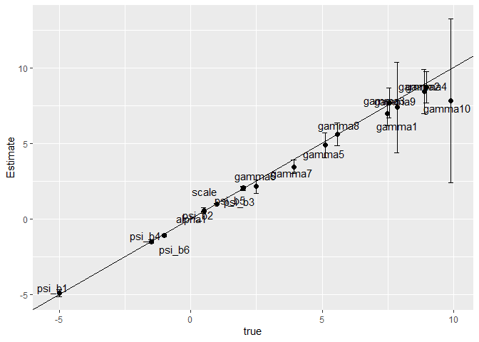
Create policy simulations (these are ‘no change’ policies with no effects)
npols <- 2 # Choose number of policies

policies <- CreateBlankPolicies(npols, mdcev_est)

df_sim <- PrepareSimulationData(mdcev_est, policies, nsims = 1)
Simulate welfare changes
wtp <- mdcev.sim(df_sim$df_indiv,
                 df_common = df_sim$df_common,
                 sim_options = df_sim$sim_options,
                 cond_err = 1,
                 nerrs = 15,
                 sim_type = "welfare")
#> Using general approach in simulation...
#>
#> 6.00e+04simulations finished in0.42minutes.(2389per second)
summary(wtp)
#> # A tibble: 2 x 5
#>   policy       mean std.dev `ci_lo2.5%` `ci_hi97.5%`
#>   <chr>       <dbl>   <dbl>       <dbl>        <dbl>
#> 1 policy1 -3.63e-11      NA   -3.63e-11    -3.63e-11
#> 2 policy2 -3.63e-11 NA -3.63e-11 -3.63e-11This package was not developed in isolation and I gratefully acknowledge Joshua Abbott, Allen Klaiber, Lusi Xie, and the apollo team whose codes or suggestions were helpful in putting this package together.