rxode2 is an R package for solving and simulating from ode-based models. These models are convert the rxode2 mini-language to C and create a compiled dll for fast solving. ODE solving using rxode2 has a few key parts:
rxode() which creates the C code for fast ODE solving
based on a simple
syntax related to Leibnitz notation.NONMEM or deSolve compatible
data frame, oret() or eventTable() for easy
simulation of eventsiCov= as needed)rxSolve() which solves the system of equations using
initial conditions and parameters to make predictions
You can install the released version of rxode2 from CRAN with:
install.packages("rxode2")You can install the development version of rxode2 with
devtools::install_github("nlmixr2/rxode2")To build models with rxode2, you need a working c compiler. To use parallel threaded solving in rxode2, this c compiler needs to support open-mp.
You can check to see if R has working c compiler you can check with:
## install.packages("pkgbuild")
pkgbuild::has_build_tools(debug = TRUE)
If you do not have the toolchain, you can set it up as described by the platform information below:
In windows you may simply use installr to install rtools:
install.packages("installr")
library(installr)
install.rtools()
Alternatively you can download and install rtools directly.
To get the most speed you need OpenMP enabled and compile rxode2 with
that compiler. There are various options and the most up to date
discussion about this is likely the data.table
installation faq for MacOS. The last thing to keep in mind is that
rxode2 uses the code very similar to the original
lsoda which requires the gfortran compiler to
be setup as well as the OpenMP compilers.
If you are going to be using rxode2 and
nlmixr together and have an older mac computer, I would
suggest trying the following:
library(symengine)If this crashes your R session then the binary does not work with
your Mac machine. To be able to run nlmixr, you will need to compile
this package manually. I will proceed assuming you have
homebrew installed on your system.
On your system terminal you will need to install the dependencies to
compile symengine:
brew install cmake gmp mpfr libmpcAfter installing the dependencies, you need to reinstall
symengine:
install.packages("symengine", type="source")
library(symengine)To install on linux make sure you install gcc (with
openmp support) and gfortran using your distribution’s
package manager.
Since the development version of rxode2 uses StanHeaders, you will need to make sure your compiler is setup to support C++14, as described in the rstan setup page. For R 4.0, I do not believe this requires modifying the windows toolchain any longer (so it is much easier to setup).
Once the C++ toolchain is setup appropriately, you can install the development version from GitHub with:
# install.packages("devtools")
devtools::install_github("nlmixr2/rxode2")The model equations can be specified through a text string, a model
file or an R expression. Both differential and algebraic equations are
permitted. Differential equations are specified by
d/dt(var_name) =. Each equation can be separated by a
semicolon.
To load rxode2 package and compile the model:
library(rxode2)
#> detected new version of rxode2, cleaning cache
#> rxode2 2.0.6 using 4 threads (see ?getRxThreads)

mod1 <- rxode2({
  C2 <- centr/V2;
  C3 <- peri/V3;
  d/dt(depot) <- -KA*depot;
  d/dt(centr) <- KA*depot - CL*C2 - Q*C2 + Q*C3;
  d/dt(peri)  <- Q*C2 - Q*C3;
  d/dt(eff)   <- Kin - Kout*(1-C2/(EC50+C2))*eff;
})
#>
#> → creating rxode2 include directory
#> → getting R compile options
#> → precompiling headers
#> ✔ doneModel parameters can be defined as named vectors. Names of parameters in the vector must be a superset of parameters in the ODE model, and the order of parameters within the vector is not important.
theta <-
   c(KA=2.94E-01, CL=1.86E+01, V2=4.02E+01, # central
     Q=1.05E+01,  V3=2.97E+02,              # peripheral
     Kin=1, Kout=1, EC50=200)               # effects
Initial conditions (ICs) can be defined through a vector as well. If the elements are not specified, the initial condition for the compartment is assumed to be zero.
inits <- c(eff=1)If you want to specify the initial conditions in the model you can add:
eff(0) = 1rxode2 provides a simple and very flexible way to
specify dosing and sampling through functions that generate an event
table. First, an empty event table is generated through the
“eventTable()” function:
ev <- eventTable(amount.units='mg', time.units='hours')Next, use the add.dosing() and
add.sampling() functions of the EventTable
object to specify the dosing (amounts, frequency and/or times, etc.) and
observation times at which to sample the state of the system. These
functions can be called multiple times to specify more complex dosing or
sampling regiments. Here, these functions are used to specify 10mg BID
dosing for 5 days, followed by 20mg QD dosing for 5 days:
ev$add.dosing(dose=10000, nbr.doses=10, dosing.interval=12)
ev$add.dosing(dose=20000, nbr.doses=5, start.time=120,
              dosing.interval=24)
ev$add.sampling(0:240)
If you wish you can also do this with the mattigr pipe
operator %>%
ev <- eventTable(amount.units="mg", time.units="hours") %>%
  add.dosing(dose=10000, nbr.doses=10, dosing.interval=12) %>%
  add.dosing(dose=20000, nbr.doses=5, start.time=120,
             dosing.interval=24) %>%
  add.sampling(0:240)
The functions get.dosing() and
get.sampling() can be used to retrieve information from the
event table.
head(ev$get.dosing())
#>   id low time high       cmt   amt rate ii addl evid ss dur
#> 1  1  NA    0   NA (default) 10000    0 12    9    1  0   0
#> 2 1 NA 120 NA (default) 20000 0 24 4 1 0 0head(ev$get.sampling())
#> id low time high cmt amt rate ii addl evid ss dur
#> 1 1 NA 0 NA (obs) NA NA NA NA 0 NA NA
#> 2 1 NA 1 NA (obs) NA NA NA NA 0 NA NA
#> 3 1 NA 2 NA (obs) NA NA NA NA 0 NA NA
#> 4 1 NA 3 NA (obs) NA NA NA NA 0 NA NA
#> 5 1 NA 4 NA (obs) NA NA NA NA 0 NA NA
#> 6 1 NA 5 NA (obs) NA NA NA NA 0 NA NAYou may notice that these are similar to NONMEM event tables; If you
are more familiar with NONMEM data and events you could use them
directly with the event table function et
ev  <- et(amountUnits="mg", timeUnits="hours") %>%
  et(amt=10000, addl=9,ii=12,cmt="depot") %>%
  et(time=120, amt=2000, addl=4, ii=14, cmt="depot") %>%
  et(0:240) # Add sampling
You can see from the above code, you can dose to the compartment named in the rxode2 model. This slight deviation from NONMEM can reduce the need for compartment renumbering.
These events can also be combined and expanded (to multi-subject
events and complex regimens) with rbind, c,
seq, and rep. For more information about
creating complex dosing regimens using rxode2 see the rxode2
events vignette.
The ODE can now be solved by calling the model object’s
run or solve function. Simulation results for
all variables in the model are stored in the output matrix x.
x <- mod1$solve(theta, ev, inits);
knitr::kable(head(x))| time | C2 | C3 | depot | centr | peri | eff |
|---|---|---|---|---|---|---|
| 0 | 0.00000 | 0.0000000 | 10000.000 | 0.000 | 0.0000 | 1.000000 |
| 1 | 44.37555 | 0.9198298 | 7452.765 | 1783.897 | 273.1895 | 1.084664 |
| 2 | 54.88296 | 2.6729825 | 5554.370 | 2206.295 | 793.8758 | 1.180825 |
| 3 | 51.90343 | 4.4564927 | 4139.542 | 2086.518 | 1323.5783 | 1.228914 |
| 4 | 44.49738 | 5.9807076 | 3085.103 | 1788.795 | 1776.2702 | 1.234610 |
| 5 | 36.48434 | 7.1774981 | 2299.255 | 1466.670 | 2131.7169 | 1.214742 |
You can also solve this and create a rxode2 data frame:
x <- mod1 %>% rxSolve(theta, ev, inits);
x
#> ── Solved rxode2 object ──
#> ── Parameters (x$params): ──
#>      V2      V3      KA      CL       Q     Kin    Kout    EC50
#>  40.200 297.000   0.294  18.600  10.500   1.000   1.000 200.000
#> ── Initial Conditions (x$inits): ──
#> depot centr  peri   eff
#>     0     0     0     1
#> ── First part of data (object): ──
#> # A tibble: 241 × 7
#>   time    C2    C3  depot centr  peri   eff
#>    [h] <dbl> <dbl>  <dbl> <dbl> <dbl> <dbl>
#> 1    0   0   0     10000     0     0   1
#> 2    1  44.4 0.920  7453. 1784.  273.  1.08
#> 3    2  54.9 2.67   5554. 2206.  794.  1.18
#> 4    3  51.9 4.46   4140. 2087. 1324.  1.23
#> 5    4  44.5 5.98   3085. 1789. 1776.  1.23
#> 6    5  36.5 7.18   2299. 1467. 2132.  1.21
#> # … with 235 more rows
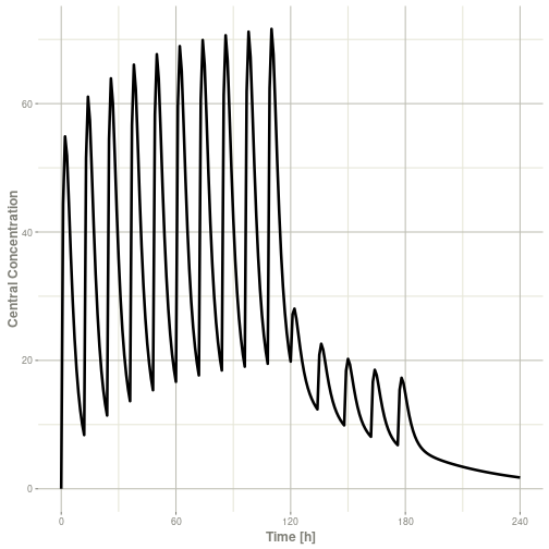
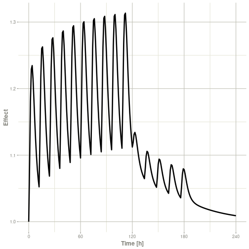
This returns a modified data frame. You can see the compartment values in the plot below:
library(ggplot2)
plot(x,C2) + ylab("Central Concentration")
Or,
plot(x,eff) + ylab("Effect")
Note that the labels are automatically labeled with the units from
the initial event table. rxode2 extracts units to label the
plot (if they are present).
This is a brief comparison of pharmacometric ODE solving R packages
to rxode2.
There are several R packages for differential equations. The most popular is deSolve.
However for pharmacometrics-specific ODE solving, there are only 2 packages other than rxode2 released on CRAN. Each uses compiled code to have faster ODE solving.
mrgsolve, which uses C++ lsoda solver to solve ODE systems. The user is required to write hybrid R/C++ code to create a mrgsolve model which is translated to C++ for solving.
In contrast, rxode2 has a R-like mini-language that is
parsed into C code that solves the ODE system.
Unlike rxode2, mrgsolve does not currently
support symbolic manipulation of ODE systems, like automatic Jacobian
calculation or forward sensitivity calculation (rxode2
currently supports this and this is the basis of nlmixr2’s FOCEi
algorithm)
dMod, which uses a unique syntax to create “reactions”. These reactions create the underlying ODEs and then created c code for a compiled deSolve model.
In contrast rxode2 defines ODE systems at a lower level.
rxode2’s parsing of the mini-language comes from C, whereas
dMod’s parsing comes from R.
Like rxode2, dMod supports symbolic
manipulation of ODE systems and calculates forward sensitivities and
adjoint sensitivities of systems.
Unlike rxode2, dMod is not thread-safe
since deSolve is not yet thread-safe.
PKPDsim which defines models in an R-like syntax and converts the system to compiled code.
Like mrgsolve, PKPDsim does not currently
support symbolic manipulation of ODE systems.
PKPDsim is not thread-safe.
The open pharmacometrics open source community is fairly friendly, and the rxode2 maintainers has had positive interactions with all of the ODE-solving pharmacometric projects listed.
rxode2 supports 1-3 compartment models with gradients
(using stan math’s auto-differentiation). This currently uses the same
equations as PKADVAN to allow time-varying covariates.
rxode2 can mix ODEs and solved systems.
mrgsolve currently has 1-2 compartment (poly-exponential models) models built-in. The solved systems and ODEs cannot currently be mixed.
pmxTools currently have 1-3 compartment (super-positioning) models built-in. This is a R-only implementation.
PKPDsim uses 1-3 “ADVAN” solutions using non-superpositioning.
PKPDmodels has a one-compartment model with gradients.