![]()
![]()
![]()
sfhotspot provides functions to identify and understand clusters of points (typically representing the locations of places or events). All the functions in the package work on and produce simple features (SF) objects, which means they can be used as part of modern spatial analysis in R.
You can install the development version of sfhotspot from GitHub with:
sfhotspot has the following functions. All can be used by just supplying an SF object containing points, or can be configured using the optional arguments to each function.
| name | use |
|---|---|
hotspot_count() |
Count the number of points in each cell of a regular grid. Cell size can be set by the user or chosen automatically. |
hotspot_kde() |
Estimate kernel density for each cell in a regular grid. Cell size and bandwidth can be set by the user or chosen automatically. |
hotspot_gistar() |
Calculate the Getis–Ord Gi* statistic for each cell in a regular grid, while optionally estimating kernel density. Cell size, bandwidth and neighbour distance can be set by the user or chosen automatically. |
There is also an included dataset memphis_robberies that contains records of 2,245 robberies in Memphis, TN, in 2019.
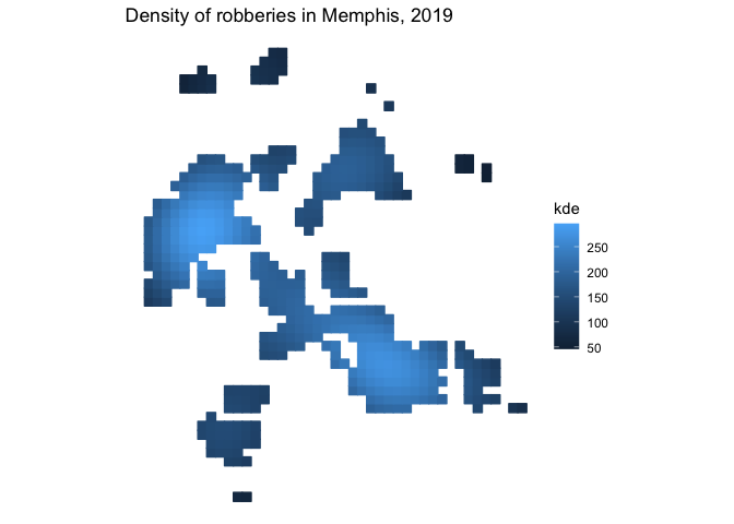
We can use the hotspot_gistar() function to identify cells in a regular grid in which there are more/fewer points than would be expected if the points were distributed randomly. In this example, the points represent the locations of personal robberies in Memphis, which is a dataset included with the package.
# Load packages
library(sf)
#> Linking to GEOS 3.9.1, GDAL 3.2.3, PROJ 7.2.1; sf_use_s2() is TRUE
library(sfhotspot)
library(tidyverse)
#> ── Attaching packages ─────────────────────────────────────── tidyverse 1.3.1 ──
#> ✓ ggplot2 3.3.5     ✓ purrr   0.3.4
#> ✓ tibble  3.1.6     ✓ dplyr   1.0.7
#> ✓ tidyr   1.2.0     ✓ stringr 1.4.0
#> ✓ readr   2.1.2     ✓ forcats 0.5.1
#> ── Conflicts ────────────────────────────────────────── tidyverse_conflicts() ──
#> x dplyr::filter() masks stats::filter()
#> x dplyr::lag()    masks stats::lag()


# Transform data to UTM zone 15N so that we can think in metres, not decimal
# degrees
memphis_robberies_utm <- st_transform(memphis_robberies, 32615)


# Identify hotspots, set all the parameters automatically by not specifying cell
# size, bandwidth, etc.
memphis_robberies_hotspots <- hotspot_gistar(memphis_robberies_utm)
#> Cell size set to 500 metres automatically
#> Bandwidth set to 5,592.453 metres automatically based on rule of thumb
#> Using centroids instead of provided `grid` geometries to calculate KDE estimates.


# Visualise the hotspots by showing only those cells that have significantly
# more points than expected by chance. For those cells, show the estimated
# density of robberies.
memphis_robberies_hotspots %>%
  filter(gistar > 0, pvalue < 0.05) %>%
  ggplot(aes(colour = kde, fill = kde)) +
  geom_sf() +
  scale_colour_continuous(aesthetics = c("colour", "fill")) +
  labs(title = "Density of robberies in Memphis, 2019") +
  theme_void()