Implementation of stability selection for graphical modelling and variable selection in regression and dimensionality reduction. These models rely on resampling approaches to estimate selection probabilities. Calibration of the hyper-parameters is done via maximisation of a stability score measuring the likelihood of informative (non-uniform) selection procedure. This package also includes tools to simulate multivariate Normal data with different (partial) correlation structures.
The development version can be downloaded from GitHub and installed using the following command from a working directory containing the folder:
devtools::install_github("barbarabodinier/sharp")We simulate data with p = 50 predictors and one outcome obtained from a linear combination of a subset of the predictors and a normally distributed error term:
library(sharp)

# Data simulation
set.seed(1)
simul <- SimulateRegression(n = 100, pk = 50)

# Predictors
X <- simul$xdata
dim(X)
#> [1] 100  50

# Continuous outcome
Y <- simul$ydata
dim(Y)
#> [1] 100   1
The output includes a binary matrix encoding if the variable was used in the outcome definition:
head(simul$theta)
#>      outcome1
#> var1        0
#> var2        0
#> var3        0
#> var4        0
#> var5        1
#> var6        0
Stability selection in a regression framework is implemented in the
function VariableSelection(). The predictor and outcome
datasets are provided as input:
stab <- VariableSelection(xdata = X, ydata = Y)print(stab)
#> Stability selection using function PenalisedRegression with gaussian family.
#> The model was run using 100 subsamples of 50% of the observations.Stability selection models with different pairs of parameters λ
(controlling the sparsity of the underlying algorithm) and π (threshold
in selection proportions) are calculated. By default, stability
selection is run in applied to LASSO regression, as implemented in
glmnet. The grids of parameter values used in the run can
be extracted using:
# First few penalty parameters
head(stab$Lambda)
#>        [,1]
#> s0 1.420237
#> s1 1.307513
#> s2 1.203736
#> s3 1.108196
#> s4 1.020239
#> s5 0.939263

# Grid of thresholds in selection proportion
stab$params$pi_list
#>  [1] 0.60 0.61 0.62 0.63 0.64 0.65 0.66 0.67 0.68 0.69 0.70 0.71 0.72 0.73 0.74
#> [16] 0.75 0.76 0.77 0.78 0.79 0.80 0.81 0.82 0.83 0.84 0.85 0.86 0.87 0.88 0.89
#> [31] 0.90

# Number of model pairs (i.e. number of visited stability selection models)
nrow(stab$Lambda) * length(stab$params$pi_list)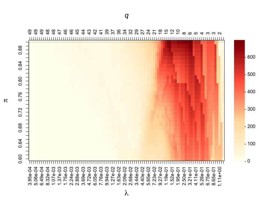
#> [1] 3100The two hyper-parameters are jointly calibrated by maximising the stability score, measuring how unlikely it is that features are uniformly selected:
par(mar = c(7, 5, 7, 6))
CalibrationPlot(stab)
Visited penalty parameters λ are represented on the x-axis. The corresponding average number of selected features by the underlying algorithm (here, LASSO regression) are reported on the z-axis and denoted by q. The different thresholds in selection proportions π are represented on the y-axis. The stability score obtained for different pairs of parameters (λ, π) are colour-coded.
The calibrated parameters and number of stably selected variables can be quickly obtained with:
summary(stab)
#> Calibrated parameters: lambda = 0.348 and pi = 0.900
#>
#> Maximum stability score: 694.140
#>
#> Number of selected variable(s): 4The stable selection status from the calibrated model can be obtained from:
SelectedVariables(stab)
#>  var1  var2  var3  var4  var5  var6  var7  var8  var9 var10 var11 var12 var13
#>     0     0     0     0     0     0     0     0     0     0     0     0     0
#> var14 var15 var16 var17 var18 var19 var20 var21 var22 var23 var24 var25 var26
#>     0     0     0     0     0     0     1     0     0     0     0     0     1
#> var27 var28 var29 var30 var31 var32 var33 var34 var35 var36 var37 var38 var39
#>     0     0     0     0     0     0     0     1     0     0     0     0     0
#> var40 var41 var42 var43 var44 var45 var46 var47 var48 var49 var50
#>     0     0     1     0     0     0     0     0     0     0     0
Stably selected variables are the ones with selection proportions above the calibrated threshold π:
plot(stab)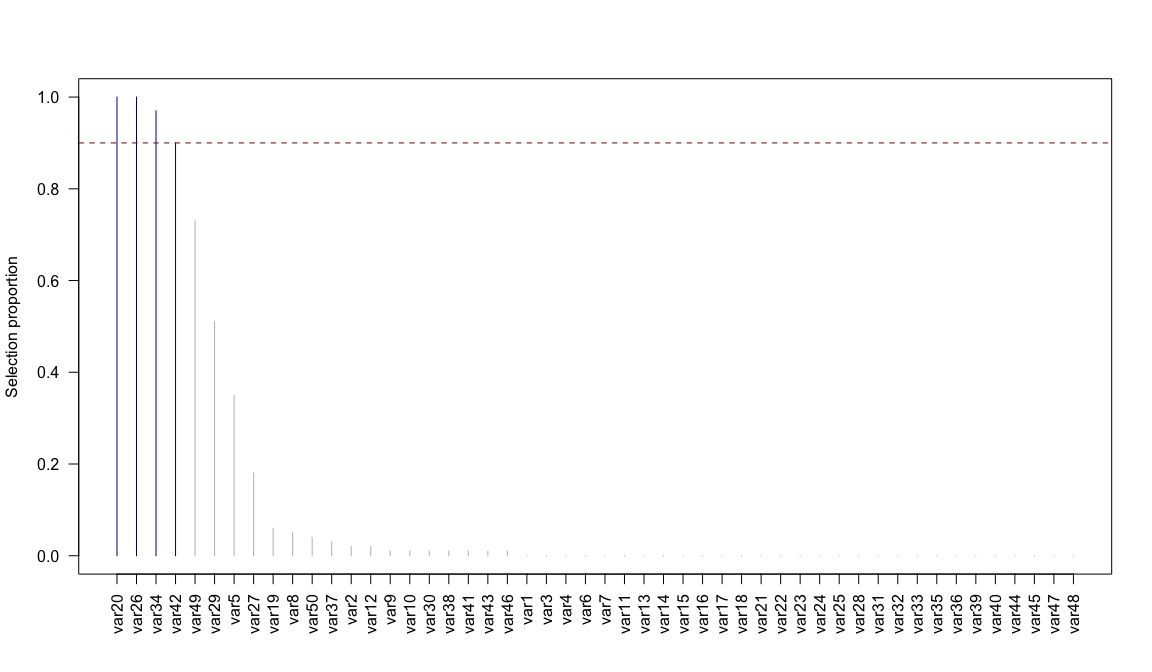
Selection proportion values can be extracted using:
SelectionProportions(stab)
#>  var1  var2  var3  var4  var5  var6  var7  var8  var9 var10 var11 var12 var13
#>  0.00  0.02  0.00  0.00  0.35  0.00  0.00  0.05  0.01  0.01  0.00  0.02  0.00
#> var14 var15 var16 var17 var18 var19 var20 var21 var22 var23 var24 var25 var26
#>  0.00  0.00  0.00  0.00  0.00  0.06  1.00  0.00  0.00  0.00  0.00  0.00  1.00
#> var27 var28 var29 var30 var31 var32 var33 var34 var35 var36 var37 var38 var39
#>  0.18  0.00  0.51  0.01  0.00  0.00  0.00  0.97  0.00  0.00  0.03  0.01  0.00
#> var40 var41 var42 var43 var44 var45 var46 var47 var48 var49 var50
#> 0.00 0.01 0.90 0.01 0.00 0.00 0.01 0.00 0.00 0.73 0.04In Gaussian Graphical Modelling, the conditional independence structure between nodes is encoded in nonzero entries of the partial correlation matrix. We simulate data with p = 10 nodes that are connected in a scale-free network, where few nodes have a lot of edges and most nodes have a small number of edges.
# Data simulation
set.seed(1)
simul <- SimulateGraphical(n = 100, pk = 10, topology = "scale-free")

# Nodes are the variables (columns)
X <- simul$data
dim(X)
#> [1] 100  10
The adjacency matrix of the simulated graph is included in the output:
simul$theta
#>       var1 var2 var3 var4 var5 var6 var7 var8 var9 var10
#> var1     0    0    0    0    0    0    0    0    1     0
#> var2     0    0    0    1    0    0    0    0    0     0
#> var3     0    0    0    0    0    0    0    0    1     1
#> var4     0    1    0    0    1    0    1    1    0     0
#> var5     0    0    0    1    0    0    0    0    0     0
#> var6     0    0    0    0    0    0    0    0    0     1
#> var7     0    0    0    1    0    0    0    0    0     0
#> var8     0    0    0    1    0    0    0    0    0     1
#> var9     1    0    1    0    0    0    0    0    0     0
#> var10    0    0    1    0    0    1    0    1    0     0
Stability selection for graphical modelling is implemented in
GraphicalModel(). For sparser estimates, the model can be
estimated under the constraint that the upper-bound of the expected
number of falsely selected edges (PFER) is below a user-defined
threshold:
stab <- GraphicalModel(xdata = X, PFER_thr = 10)print(stab)
#> Stability selection using function PenalisedGraphical.
#> The model was run using 100 subsamples of 50% of the observations.As in variable selection, parameters are jointly calibrated by maximising the stability score:
par(mar = c(7, 5, 7, 6))
CalibrationPlot(stab)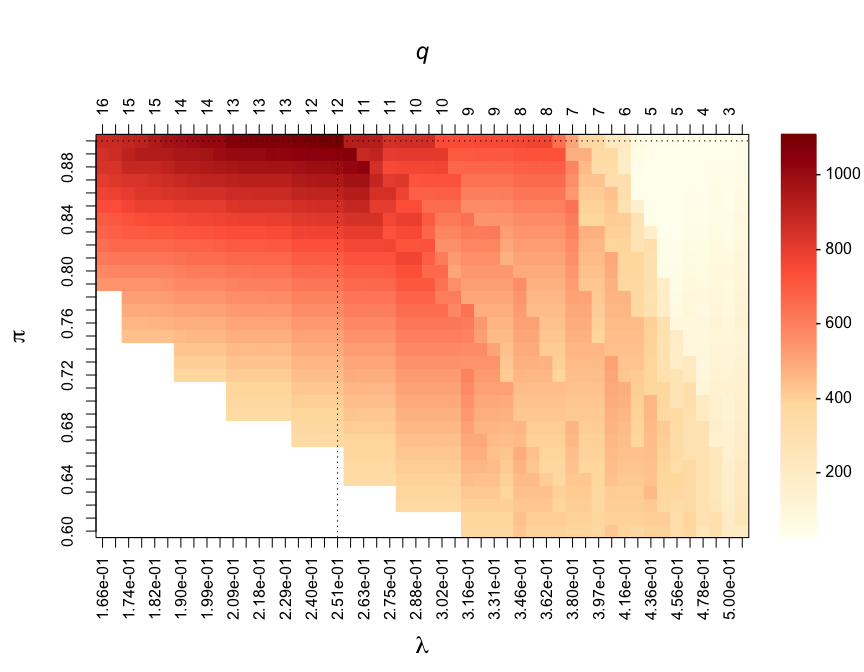
The effect of the constraint on the PFER can be visualised in this calibration plot. The white area corresponds to “forbidden” models, where the upper-bound of the expected number of parameters would exceed the value specified in PFER_thr.
Calibrated parameters and number of edges in the calibrated model can be viewed using:
summary(stab)
#> Calibrated parameters: lambda = 0.251 and pi = 0.900
#>
#> Maximum stability score: 1102.130
#>
#> Number of selected edge(s): 9The calibrated graph can be visualised using:
set.seed(1)
plot(stab)
The adjacency matrix of the calibrated stability selection graphical model can be extracted using:
Adjacency(stab)
#>       var1 var2 var3 var4 var5 var6 var7 var8 var9 var10
#> var1     0    0    0    0    0    0    0    0    1     0
#> var2     0    0    0    1    0    0    0    0    0     0
#> var3     0    0    0    0    0    0    0    0    1     1
#> var4     0    1    0    0    1    0    1    1    0     0
#> var5     0    0    0    1    0    0    0    0    0     0
#> var6     0    0    0    0    0    0    0    0    0     1
#> var7     0    0    0    1    0    0    0    0    0     0
#> var8     0    0    0    1    0    0    0    0    0     1
#> var9     1    0    1    0    0    0    0    0    0     0
#> var10    0    0    1    0    0    1    0    1    0     0
And converted to an igraph object using:
mygraph=Graph(Adjacency(stab))
set.seed(1)
plot(mygraph)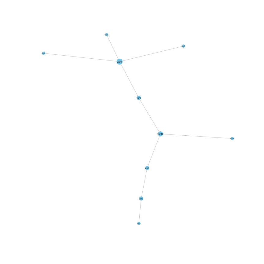
We simulate data with p = 12 variables related to N = 3 latent variables:
# Data simulation
set.seed(1)
simul <- SimulateComponents(n = 100, pk = c(3, 5, 4), v_within = c(0.8, 1), v_sign = -1)
#> The smallest proportion of explained variance by PC1 that can be obtained is 0.24.

# Simulated data
X <- simul$data

# Pearson's correlations
plot(simul)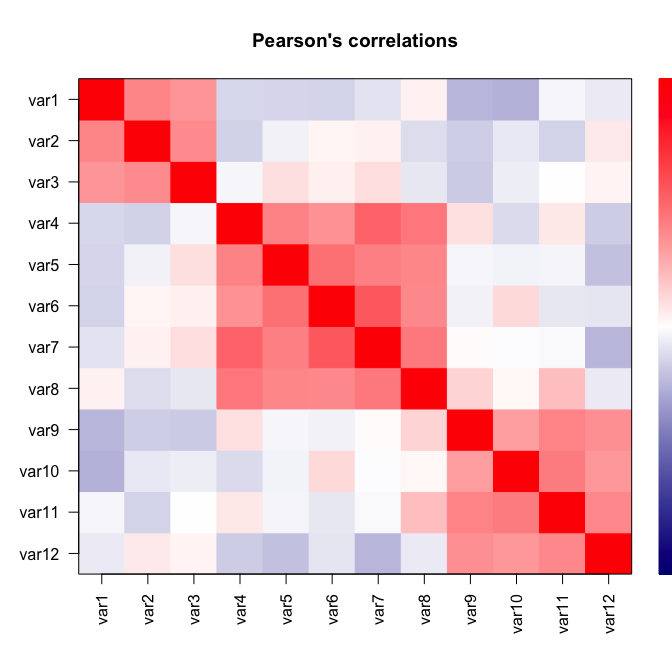
# Relationships between variables and latent variables
simul$theta
#>       comp1 comp2 comp3 comp4 comp5 comp6 comp7 comp8 comp9 comp10 comp11
#> var1      0     0     1     1     1     0     0     0     0      0      0
#> var2      0     0     1     1     1     0     0     0     0      0      0
#> var3      0     0     1     1     1     0     0     0     0      0      0
#> var4      1     0     0     0     0     0     0     0     1      1      1
#> var5      1     0     0     0     0     0     0     0     1      1      1
#> var6      1     0     0     0     0     0     0     0     1      1      1
#> var7      1     0     0     0     0     0     0     0     1      1      1
#> var8      1     0     0     0     0     0     0     0     1      1      1
#> var9      0     1     0     0     0     1     1     1     0      0      0
#> var10     0     1     0     0     0     1     1     1     0      0      0
#> var11     0     1     0     0     0     1     1     1     0      0      0
#> var12     0     1     0     0     0     1     1     1     0      0      0
#>       comp12
#> var1       0
#> var2       0
#> var3       0
#> var4       1
#> var5       1
#> var6       1
#> var7       1
#> var8       1
#> var9       0
#> var10      0
#> var11      0
#> var12      0
Stability selection for dimensionality reduction is implemented in
BiSelection(). It can be used in combination with sparse
Principal Component Analysis (sPCA) to recover the sparse set of
variables contributing to the Principal Components (PCs). Stability
selection can be applied on the first three PCs using:
stab <- BiSelection(xdata = X, implementation = SparsePCA, ncomp = 3)
#> Component 1
#> Loading required namespace: elasticnet
#> Component 2
#> Component 3print(stab)
#> Stability selection using function SparsePCA with gaussian family.
#> The model was run using 100 subsamples of 50% of the observations.As for models presented in previous sections, the hyper-parameters are calibrated by maximising the stability score.
par(mar = c(7, 5, 7, 6))
CalibrationPlot(stab)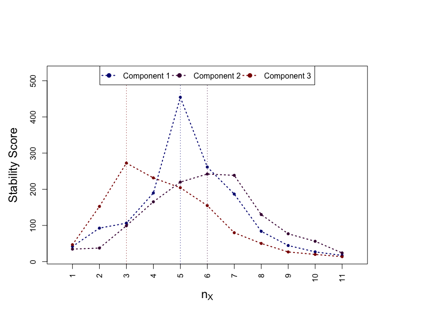
The PC-specific calibrated parameters are reported in:
stab$summary
#>   comp nx  pix        S
#> 1    1  5 0.90 454.4235
#> 2    2  6 0.88 242.0888
#> 3 3 3 0.84 272.4526The sets of stably selected variables for each of the PCs are encoded in:
SelectedVariables(stab)
#>       comp1 comp2 comp3
#> var1      0     0     1
#> var2      0     0     1
#> var3      0     0     1
#> var4      1     0     0
#> var5      1     0     0
#> var6      1     0     0
#> var7      1     0     0
#> var8      1     0     0
#> var9      0     1     0
#> var10     0     1     0
#> var11     0     1     0
#> var12     0     0     0
This can be visualised in a network:
set.seed(1)
plot(stab)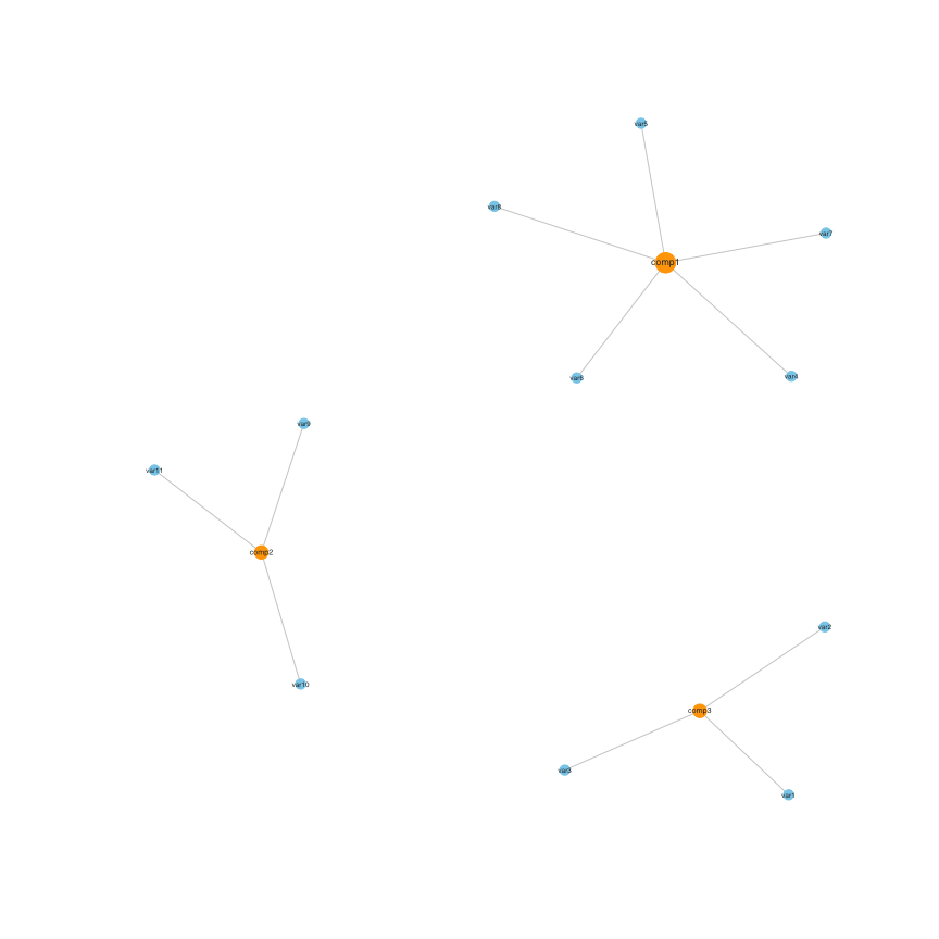
Corresponding selection proportions for each of the three PCs can be obtained from:
SelectionProportions(stab)
#>       comp1 comp2 comp3
#> var1   0.08  0.76  0.84
#> var2   0.05  0.68  0.86
#> var3   0.00  0.42  0.87
#> var4   0.91  0.09  0.01
#> var5   0.91  0.09  0.00
#> var6   0.92  0.10  0.01
#> var7   0.91  0.11  0.00
#> var8   0.93  0.21  0.00
#> var9   0.08  0.91  0.07
#> var10  0.08  0.88  0.06
#> var11  0.07  0.90  0.13
#> var12  0.06  0.85  0.15