![]()
This package creates short sprint (<6sec) profiles using the split times, or the radar gun data. Mono-exponential equation is used to estimate maximal sprinting speed (MSS), relative acceleration (TAU), and other parameters. These parameters can be used to predict kinematic and kinetics variables and to compare individuals.
# Install from CRAN
install.packages("shorts")

# Or the development version from GitHub
# install.packages("devtools")
devtools::install_github("mladenjovanovic/shorts"){shorts} comes with two sample data sets: split_times
and radar_gun_data with N=5 athletes. Let’s load them
both:
require(shorts)
require(tidyverse)
require(knitr)

data("split_times", "radar_gun_data")To model sprint performance using split times, distance will be used
as predictor and time as target. Since split_times contains
data for multiple athletes, let’s extract only one athlete and model it
using shorts::model_timing_gates() function.
kimberley_data <- filter(split_times, athlete == "Kimberley")

kable(kimberley_data)| athlete | bodyweight | distance | time |
|---|---|---|---|
| Kimberley | 55 | 5 | 1.158 |
| Kimberley | 55 | 10 | 1.893 |
| Kimberley | 55 | 15 | 2.541 |
| Kimberley | 55 | 20 | 3.149 |
| Kimberley | 55 | 30 | 4.313 |
| Kimberley | 55 | 40 | 5.444 |
shorts::model_timing_gates() returns an object with
parameters, model_fit, model
returned from minpack.lm::nlsLM() function and
data used to estimate parameters. Parameters estimated
using mono-exponential equation are maximal sprinting speed
(MSS), and relative acceleration (TAU). Additional parameters
computed from MSS and TAU are maximal acceleration (MAC) and
maximal relative power (PMAX) (which is calculated as
MAC*MSS/4).
kimberley_profile <- shorts::model_timing_gates(
  distance = kimberley_data$distance,
  time = kimberley_data$time)

kimberley_profile
#> Estimated model parameters
#> --------------------------
#>    MSS    TAU    MAC   PMAX
#>  8.591  0.811 10.589 22.743
#>
#> Model fit estimators
#> --------------------
#>       RSE R_squared    minErr    maxErr maxAbsErr      RMSE       MAE      MAPE
#>    0.0340    0.9997   -0.0529    0.0270    0.0529    0.0278    0.0233    1.1926

summary(kimberley_profile)
#>
#> Formula: time ~ TAU * I(LambertW::W(-exp(1)^(-distance/(MSS * TAU) - 1))) +
#>     distance/MSS + TAU
#>
#> Parameters:
#>     Estimate Std. Error t value Pr(>|t|)
#> MSS   8.5911     0.1225    70.1  2.5e-07 ***
#> TAU   0.8113     0.0458    17.7  6.0e-05 ***
#> ---
#> Signif. codes:  0 '***' 0.001 '**' 0.01 '*' 0.05 '.' 0.1 ' ' 1
#>
#> Residual standard error: 0.034 on 4 degrees of freedom
#>
#> Number of iterations to convergence: 5
#> Achieved convergence tolerance: 1.49e-08

coef(kimberley_profile)
#>    MSS    TAU    MAC   PMAX
#>  8.591  0.811 10.589 22.743
To return the predicted outcome (in this case time variable), use
predict() function:
predict(kimberley_profile)
#> [1] 1.21 1.90 2.52 3.12 4.30 5.47
To create a simple plot, use S3 plot() method:
plot(kimberley_profile) +
  theme_bw()
If you are interested in calculating average split velocity, use
shorts::format_splits()
kable(shorts::format_splits(
  distance = kimberley_data$distance,
time = kimberley_data$time))| split | split_distance_start | split_distance_stop | split_distance | split_time_start | split_time_stop | split_time | split_mean_velocity |
|---|---|---|---|---|---|---|---|
| 1 | 0 | 5 | 5 | 0 | 1.158 | 1.158 | 4.317789…. |
| 2 | 5 | 10 | 5 | 1.158 | 1.893 | 0.735 | 6.802721…. |
| 3 | 10 | 15 | 5 | 1.893 | 2.541 | 0.648 | 7.716049…. |
| 4 | 15 | 20 | 5 | 2.541 | 3.149 | 0.608 | 8.223684…. |
| 5 | 20 | 30 | 10 | 3.149 | 4.313 | 1.164 | 8.591065…. |
| 6 | 30 | 40 | 10 | 4.313 | 5.444 | 1.131 | 8.841732…. |
Let’s plot observed vs fitted split times. For this we can use
data returned from
shorts::model_timing_gates() since it contains
pred_time column.
ggplot(kimberley_profile$data, aes(x = distance)) +
  theme_bw() +
  geom_point(aes(y = time)) +
  geom_line(aes(y = pred_time)) +
  xlab("Distance (m)") +
  ylab("Time (s)")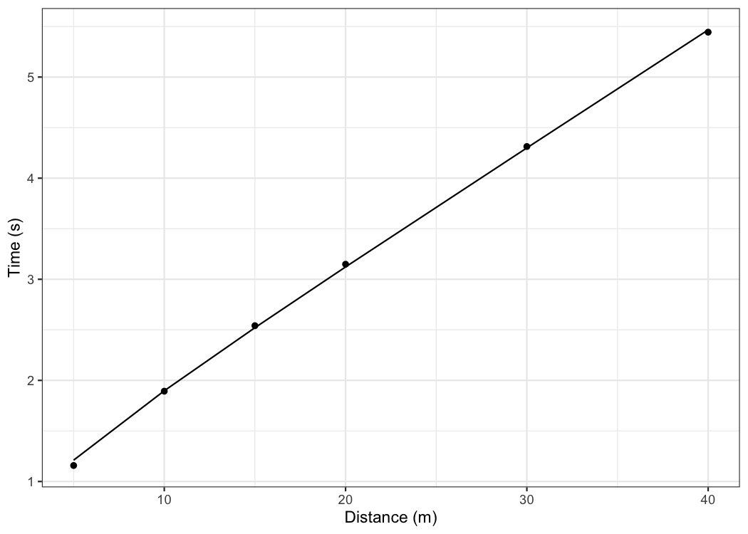
To plot predicted velocity, acceleration, air resistance, force, and
power over distance, use shorts:predict_XXX(). Please note
that to calculate force, air resistance, and power, we need Kimberley’s
bodymass and height (as well as other characteristics such as air
pressure, temperature and wind - see get_air_resistance()
function).
kimberley_bodymass <- 60 # in kilograms
kimberley_bodyheight <- 1.7 # in meters

kimberley_pred <- tibble(
  distance = seq(0, 40, length.out = 1000),

  # Velocity
  pred_velocity = shorts::predict_velocity_at_distance(
    distance,
    kimberley_profile$parameters$MSS,
    kimberley_profile$parameters$TAU),

  # Acceleration
  pred_acceleration = shorts::predict_acceleration_at_distance(
    distance,
    kimberley_profile$parameters$MSS,
    kimberley_profile$parameters$TAU),

  # Air resistance
  pred_air_resistance = shorts::predict_air_resistance_at_distance(
    distance,
    kimberley_profile$parameters$MSS,
    kimberley_profile$parameters$TAU,
    bodymass = kimberley_bodymass,
    bodyheight = kimberley_bodyheight),

  # Force
  pred_force = shorts::predict_force_at_distance(
    distance,
    kimberley_profile$parameters$MSS,
    kimberley_profile$parameters$TAU,
    bodymass = kimberley_bodymass,
    bodyheight = kimberley_bodyheight),

  # Power
  pred_power = shorts::predict_power_at_distance(
    distance,
    kimberley_profile$parameters$MSS,
    kimberley_profile$parameters$TAU,
    bodymass = kimberley_bodymass,
    bodyheight = kimberley_bodyheight),
)

# Convert to long
kimberley_pred <- gather(kimberley_pred, "metric", "value", -distance)

ggplot(kimberley_pred, aes(x = distance, y = value)) +
  theme_bw() +
  geom_line() +
  facet_wrap(~metric, scales = "free_y") +
  xlab("Distance (m)") +
  ylab(NULL)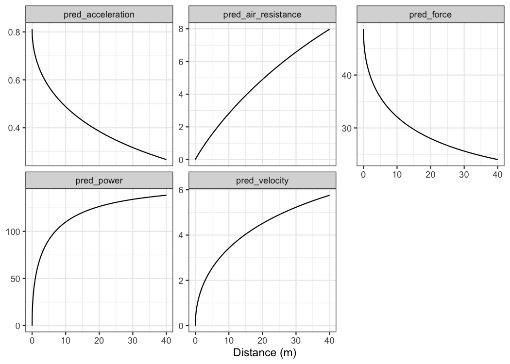
To do prediction simpler, use
shorts::predict_kinematics() function. This will provide
kinetics and kinematics for 0-6s sprint using 100Hz.
predicted_kinematics <- predict_kinematics(
  kimberley_profile,
  bodymass = kimberley_bodymass,
  bodyheight = kimberley_bodyheight)

kable(head(predicted_kinematics))| time | distance | velocity | acceleration | bodymass | net_horizontal_force | air_resistance | horizontal_force | horizontal_force_relative | vertical_force | resultant_force | resultant_force_relative | power | relative_power | RF | force_angle |
|---|---|---|---|---|---|---|---|---|---|---|---|---|---|---|---|
| 0.00 | 0.000 | 0.000 | 10.59 | 60 | 635 | 0.000 | 635 | 10.59 | 589 | 866 | 14.4 | 0 | 0.00 | 0.734 | 42.8 |
| 0.01 | 0.001 | 0.105 | 10.46 | 60 | 628 | 0.003 | 628 | 10.46 | 589 | 860 | 14.3 | 66 | 1.10 | 0.729 | 43.2 |
| 0.02 | 0.002 | 0.209 | 10.33 | 60 | 620 | 0.011 | 620 | 10.33 | 589 | 855 | 14.2 | 130 | 2.16 | 0.725 | 43.5 |
| 0.03 | 0.005 | 0.312 | 10.21 | 60 | 612 | 0.023 | 612 | 10.21 | 589 | 849 | 14.2 | 191 | 3.18 | 0.721 | 43.9 |
| 0.04 | 0.008 | 0.413 | 10.08 | 60 | 605 | 0.041 | 605 | 10.08 | 589 | 844 | 14.1 | 250 | 4.17 | 0.717 | 44.2 |
| 0.05 | 0.013 | 0.513 | 9.96 | 60 | 597 | 0.063 | 597 | 9.96 | 589 | 839 | 14.0 | 307 | 5.11 | 0.712 | 44.6 |
To get model residuals, use residuals() function:
residuals(kimberley_profile)
#> [1] -0.05293 -0.00402  0.01997  0.02699  0.01376 -0.02232
Package {shorts} comes with find_XXX() family of
functions that allow finding peak power and it’s location, as well as
critical distance over which velocity, acceleration, or power
drops below certain threshold:
# Peak power and location
shorts::find_max_power_distance(
  kimberley_profile$parameters$MSS,
  kimberley_profile$parameters$TAU
)
#> $max_power
#> [1] 172
#>
#> $distance
#> [1] 100

# Distance over which power is over 50%
shorts::find_power_critical_distance(
  MSS = kimberley_profile$parameters$MSS,
  MAC = kimberley_profile$parameters$MAC,
  percent = 0.5
)
#> $lower
#> [1] 0.0856
#>
#> $upper
#> [1] 8.36

# Distance over which acceleration is under 50%
shorts::find_acceleration_critical_distance(
  MSS = kimberley_profile$parameters$MSS,
  MAC = kimberley_profile$parameters$MAC,
  percent = 0.5
)
#> [1] 1.35

# Distance over which velocity is over 95%
shorts::find_velocity_critical_distance(
  MSS = kimberley_profile$parameters$MSS,
  MAC = kimberley_profile$parameters$MAC,
  percent = 0.95
)
#> [1] 14.3The radar gun data is modeled using measured velocity as target
variable and time as predictor. Individual analysis is performed using
shorts::model_radar_gun() function. Let’s do analysis for
Jim:
jim_data <- filter(radar_gun_data, athlete == "Jim")

jim_profile <- shorts::model_radar_gun(
  time = jim_data$time,
  velocity = jim_data$velocity
)

jim_profile
#> Estimated model parameters
#> --------------------------
#>      MSS      TAU      MAC     PMAX       TC
#>  7.99801  0.88880  8.99871 17.99294  0.00011
#>
#> Model fit estimators
#> --------------------
#>       RSE R_squared    minErr    maxErr maxAbsErr      RMSE       MAE      MAPE
#>    0.0506    0.9992   -0.1640    0.1511    0.1640    0.0505    0.0393       Inf

summary(jim_profile)
#>
#> Formula: velocity ~ MSS * (1 - exp(1)^(-(time + TC)/TAU))
#>
#> Parameters:
#>     Estimate Std. Error t value Pr(>|t|)
#> MSS  7.99801    0.00319 2504.54   <2e-16 ***
#> TAU  0.88880    0.00218  407.81   <2e-16 ***
#> TC   0.00011    0.00123    0.09     0.93
#> ---
#> Signif. codes:  0 '***' 0.001 '**' 0.01 '*' 0.05 '.' 0.1 ' ' 1
#>
#> Residual standard error: 0.0506 on 597 degrees of freedom
#>
#> Number of iterations to convergence: 4
#> Achieved convergence tolerance: 1.49e-08

plot(jim_profile) +
  theme_bw()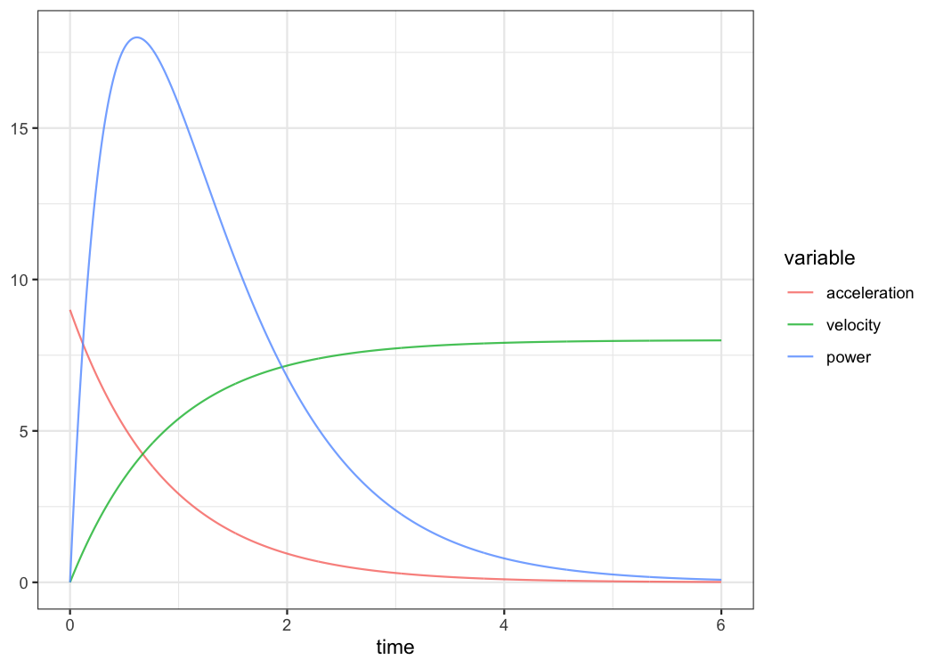
The object returned from shorts::model_radar_gun() is
same as object returned from shorts::model_timing_gates().
Let’s plot Jim’s measured velocity and predicted velocity:
ggplot(jim_profile$data, aes(x = time)) +
  theme_bw() +
  geom_line(aes(y = velocity), alpha = 0.5) +
  geom_line(aes(y = pred_velocity), color = "red", alpha = 0.5) +
  xlab("Time (s)") +
  ylab("Velocity (m/s)")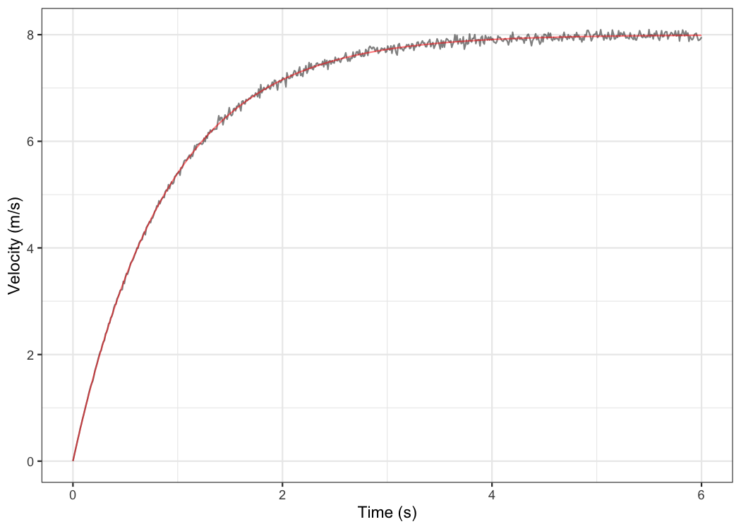
To estimate Force-Velocity profile using approach by Samozino et
al. (2016), use shorts::make_FV_profile():
kimberley_fv <- shorts::make_FV_profile(
  MSS = kimberley_profile$parameters$MSS,
  MAC = kimberley_profile$parameters$MAC,
  # These are needed to estimate air resistance
  bodymass = kimberley_bodymass,
  bodyheight = kimberley_bodyheight
)

kimberley_fv
#> Estimated Force-Velocity Profile
#> --------------------------------
#>      bodymass            F0        F0_rel            V0          Pmax
#>      6.00e+01      6.30e+02      1.05e+01      8.83e+00      1.39e+03
#> Pmax_relative      FV_slope  RFmax_cutoff         RFmax           Drf
#>      2.32e+01     -1.19e+00      3.00e-01      5.99e-01     -1.04e-01
#>        RSE_FV       RSE_Drf
#>      9.95e-01      9.46e-03

plot(kimberley_fv) +
  theme_bw()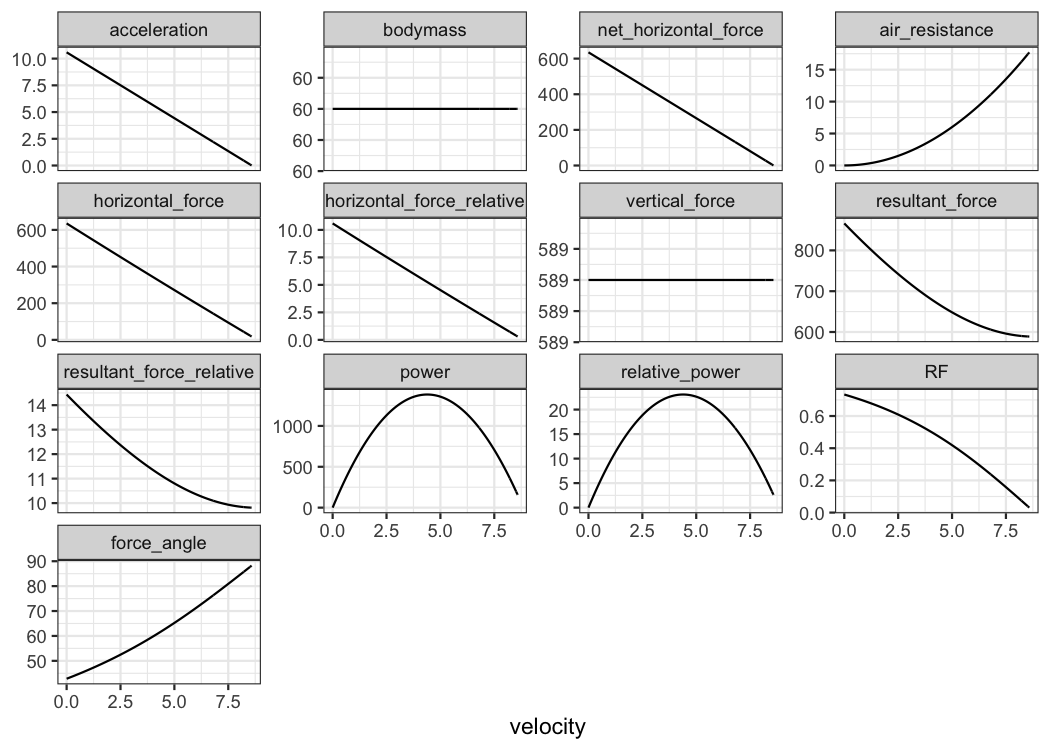
You have probably noticed that estimated MSS and TAU were a bit too high for splits data. Biased estimates are due to differences in starting positions and timing triggering methods for certain measurement approaches (e.g. starting behind first timing gate, or allowing for body rocking).
Here I will provide quick summary. Often, this bias in estimates is
dealt with by using heuristic rule of thumb of adding time correction
(time_correction) to split times (e.g. from 0.3-0.5sec; see
more in Haugen et al., 2012). To do this, just add time
correction to time split:
kimberley_profile_fixed_TC <- shorts::model_timing_gates(
  distance = kimberley_data$distance,
  time = kimberley_data$time + 0.3)

kimberley_profile_fixed_TC
#> Estimated model parameters
#> --------------------------
#>   MSS   TAU   MAC  PMAX
#>  9.13  1.38  6.63 15.12
#>
#> Model fit estimators
#> --------------------
#>       RSE R_squared    minErr    maxErr maxAbsErr      RMSE       MAE      MAPE
#>   0.00997   0.99997  -0.00769   0.01640   0.01640   0.00814   0.00639   0.28570

summary(kimberley_profile_fixed_TC)
#>
#> Formula: time ~ TAU * I(LambertW::W(-exp(1)^(-distance/(MSS * TAU) - 1))) +
#>     distance/MSS + TAU
#>
#> Parameters:
#>     Estimate Std. Error t value Pr(>|t|)
#> MSS   9.1278     0.0536   170.4  7.1e-09 ***
#> TAU   1.3776     0.0213    64.7  3.4e-07 ***
#> ---
#> Signif. codes:  0 '***' 0.001 '**' 0.01 '*' 0.05 '.' 0.1 ' ' 1
#>
#> Residual standard error: 0.00997 on 4 degrees of freedom
#>
#> Number of iterations to convergence: 5
#> Achieved convergence tolerance: 1.49e-08

coef(kimberley_profile_fixed_TC)
#>   MSS   TAU   MAC  PMAX
#>  9.13  1.38  6.63 15.12
Instead of providing for TC, this parameter can be
estimated using shorts::model_timing_gates_TC().
kimberley_profile_TC <- shorts::model_timing_gates_TC(
  distance = kimberley_data$distance,
  time = kimberley_data$time)

kimberley_profile_TC
#> Estimated model parameters
#> --------------------------
#>    MSS    TAU    MAC   PMAX     TC
#>  8.975  1.235  7.268 16.307  0.235
#>
#> Model fit estimators
#> --------------------
#>       RSE R_squared    minErr    maxErr maxAbsErr      RMSE       MAE      MAPE
#>  0.001129  1.000000 -0.001181  0.001209  0.001209  0.000798  0.000659  0.028235
Instead of estimating TC, {shorts} package features a
method of estimating flying start distance (FD):
kimberley_profile_FD <- shorts::model_timing_gates_FD(
  distance = kimberley_data$distance,
  time = kimberley_data$time)

kimberley_profile_FD
#> Estimated model parameters
#> --------------------------
#>    MSS    TAU    MAC   PMAX     FD
#>  9.003  1.288  6.991 15.735  0.302
#>
#> Model fit estimators
#> --------------------
#>       RSE R_squared    minErr    maxErr maxAbsErr      RMSE       MAE      MAPE
#> 0.000390 1.000000 -0.000404 0.000456 0.000456 0.000276 0.000237 0.007829model_timing_gates_() family of functions come with
LOOCV feature that is performed by setting the function parameter
LOOCV = TRUE. This feature is very useful for checking
model parameters robustness and model predictions on unseen data. LOOCV
involve iterative model building and testing by removing observation one
by one and making predictions for them. Let’s use Kimberley again, but
this time perform LOOCV:
kimberley_profile_LOOCV <- shorts::model_timing_gates(
  distance = kimberley_data$distance,
  time = kimberley_data$time,
  LOOCV = TRUE)

kimberley_profile_LOOCV
#> Estimated model parameters
#> --------------------------
#>    MSS    TAU    MAC   PMAX
#>  8.591  0.811 10.589 22.743
#>
#> Model fit estimators
#> --------------------
#>       RSE R_squared    minErr    maxErr maxAbsErr      RMSE       MAE      MAPE
#>    0.0340    0.9997   -0.0529    0.0270    0.0529    0.0278    0.0233    1.1926
#>
#>
#> Cross-Validation
#> ------------------------------
#> Parameters:
#> # A tibble: 6 × 4
#>     MSS   TAU   MAC  PMAX
#>   <dbl> <dbl> <dbl> <dbl>
#> 1  8.69 0.856  10.2  22.1
#> 2  8.60 0.815  10.5  22.7
#> 3  8.56 0.795  10.8  23.0
#> 4  8.57 0.797  10.8  23.0
#> 5  8.61 0.813  10.6  22.8
#> 6  8.39 0.760  11.1  23.2
#>
#> Testing model fit:
#>       RSE R_squared    minErr    maxErr maxAbsErr      RMSE       MAE      MAPE
#>        NA    0.9990   -0.0801    0.0344    0.0801    0.0474    0.0392    1.7227
Box-plot is suitable method for plotting estimated parameters:
LOOCV_parameters <- gather(kimberley_profile_LOOCV$CV$parameters)

ggplot(LOOCV_parameters, aes(y = value)) +
  theme_bw() +
  geom_boxplot() +
  facet_wrap(~key, scales = "free") +
  ylab(NULL) +
  theme(axis.ticks.x = element_blank(), axis.text.x = element_blank())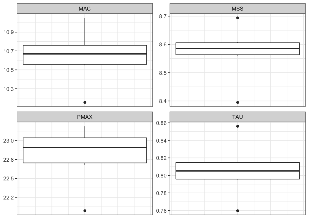
Let’s plot model LOOCV predictions and training (when using all data set) predictions against observed performance:
kimberley_data <- kimberley_data %>%
  mutate(
    pred_time = predict(kimberley_profile_LOOCV),
    LOOCV_time = kimberley_profile_LOOCV$CV$data$pred_time
  )

ggplot(kimberley_data, aes(x = distance)) +
  theme_bw() +
  geom_point(aes(y = time)) +
  geom_line(aes(y = pred_time), color = "black") +
  geom_line(aes(y = LOOCV_time), color = "red") +
  xlab("Distance (m)") +
  ylab("Time (s)")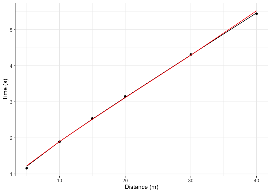
Let’s plot predicted velocity using LOOCV estimate parameters to check robustness of the model predictions:
plot_data <- kimberley_profile_LOOCV$CV$parameters %>%
  mutate(LOOCV = row_number())

plot_data <- expand_grid(
  data.frame(time = seq(0, 6, length.out = 100)),
  plot_data
) %>%
  mutate(
    LOOCV_velocity = predict_velocity_at_time(
      time = time,
      MSS = MSS,
      MAC = MAC),
    velocity = predict_velocity_at_time(
      time = time,
      MSS = kimberley_profile_LOOCV$parameters$MSS,
      MAC = kimberley_profile_LOOCV$parameters$MAC)
  )

ggplot(plot_data, aes(x = time, y = LOOCV_velocity, group = LOOCV)) +
  theme_bw() +
  geom_line(alpha = 0.8) +
  geom_line(aes(y = velocity), color = "red", size = 0.5) +
  xlab("Time (sec)") +
  ylab("Velocity (m/s)")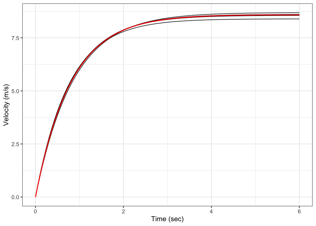
Cross-validation implemented in model_radar_gun()
function involves using n-folds, set by using CV=
parameter:
jim_profile_CV <- shorts::model_radar_gun(
  time = jim_data$time,
  velocity = jim_data$velocity,
  CV = 10
)

jim_profile_CV
#> Estimated model parameters
#> --------------------------
#>      MSS      TAU      MAC     PMAX       TC
#>  7.99801  0.88880  8.99871 17.99294  0.00011
#>
#> Model fit estimators
#> --------------------
#>       RSE R_squared    minErr    maxErr maxAbsErr      RMSE       MAE      MAPE
#>    0.0506    0.9992   -0.1640    0.1511    0.1640    0.0505    0.0393       Inf
#>
#>
#> Cross-Validation
#> ------------------------------
#> Parameters:
#> # A tibble: 10 × 5
#>      MSS   TAU   MAC  PMAX         TC
#>    <dbl> <dbl> <dbl> <dbl>      <dbl>
#>  1  8.00 0.889  8.99  18.0  0.000230
#>  2  8.00 0.889  8.99  18.0  0.000374
#>  3  8.00 0.889  9.00  18.0  0.0000424
#>  4  8.00 0.888  9.01  18.0 -0.000197
#>  5  8.00 0.889  9.00  18.0  0.000129
#>  6  8.00 0.889  9.00  18.0  0.000113
#>  7  8.00 0.889  9.00  18.0  0.000192
#>  8  8.00 0.889  9.00  18.0  0.000104
#>  9  8.00 0.889  8.99  18.0  0.000271
#> 10  8.00 0.888  9.00  18.0 -0.000141
#>
#> Testing model fit:
#>       RSE R_squared    minErr    maxErr maxAbsErr      RMSE       MAE      MAPE
#> NA 0.9992 -0.1638 0.1524 0.1638 0.0506 0.0393 InfJovanović, M., Vescovi, J.D. (2020). shorts: An R Package for Modeling Short Sprints. Preprint available at SportRxiv. https://doi.org/10.31236/osf.io/4jw62
Vescovi, JD and Jovanović, M. Sprint Mechanical Characteristics of Female Soccer Players: A Retrospective Pilot Study to Examine a Novel Approach for Correction of Timing Gate Starts. Front Sports Act Living 3: 629694, 2021. https://doi.org/10.3389/fspor.2021.629694
To cite {shorts}, please use the following command to get the BibTex entry:
citation("shorts")Please refer to these publications for more information on short
sprints modeling using mono-exponential equation, as well as on
performing mixed non-linear models with nlme package:
Chelly SM, Denis C. 2001. Leg power and hopping stiffness: relationship with sprint running performance: Medicine and Science in Sports and Exercise:326–333. DOI: 10.1097/00005768-200102000-00024.
Clark KP, Rieger RH, Bruno RF, Stearne DJ. 2017. The NFL Combine 40-Yard Dash: How Important is Maximum Velocity? Journal of Strength and Conditioning Research:1. DOI: 10.1519/JSC.0000000000002081.
Furusawa K, Hill AV, and Parkinson JL. The dynamics of” sprint” running. Proceedings of the Royal Society of London. Series B, Containing Papers of a Biological Character 102 (713): 29-42, 1927
Greene PR. 1986. Predicting sprint dynamics from maximum-velocity measurements. Mathematical Biosciences 80:1–18. DOI: 10.1016/0025-5564(86)90063-5.
Haugen TA, Tønnessen E, Seiler SK. 2012. The Difference Is in the Start: Impact of Timing and Start Procedure on Sprint Running Performance: Journal of Strength and Conditioning Research 26:473–479. DOI: 10.1519/JSC.0b013e318226030b.
Pinheiro J, Bates D, DebRoy S, Sarkar D, R Core Team. 2019. nlme: Linear and nonlinear mixed effects models.
Samozino P, Rabita G, Dorel S, Slawinski J, Peyrot N, Saez de Villarreal E, Morin J-B. 2016. A simple method for measuring power, force, velocity properties, and mechanical effectiveness in sprint running: Simple method to compute sprint mechanics. Scandinavian Journal of Medicine & Science in Sports 26:648–658. DOI: 10.1111/sms.12490.
Samozino P. 2018. A Simple Method for Measuring Force, Velocity and Power Capabilities and Mechanical Effectiveness During Sprint Running. In: Morin J-B, Samozino P eds. Biomechanics of Training and Testing. Cham: Springer International Publishing, 237–267. DOI: 10.1007/978-3-319-05633-3_11.