spatial_power
|
Main function. Compute the statistical power of a spatial relative risk function using randomly generated data.
|
spatial_data
|
Generate random bivariate data for a spatial relative risk function.
|
jitter_power
|
Compute the statistical power of a spatial relative risk function using previously collected data.
|
spatial_plots
|
Easily make multiple plots from spatial_power, spatial_data, and jitter_power outputs.
|
pval_correct
|
Called within spatial_power and jitter_power, calculates various multiple testing corrections for the alpha level.
|
Authors
Ian D. Buller - Occupational and Environmental Epidemiology Branch, Division of Cancer Epidemiology and Genetics, National Cancer Institute, National Institutes of Health, Rockville, Maryland - GitHub
Derek W. Brown - Integrative Tumor Epidemiology Branch, Division of Cancer Epidemiology and Genetics, National Cancer Institute, National Institutes of Health, Rockville, Maryland - GitHub
See also the list of contributors who participated in this package, including:
- Tim A. Myers - Laboratory of Genetic Susceptibility, Division of Cancer Epidemiology and Genetics, National Cancer Institute, National Institutes of Health, Rockville, Maryland - GitHub
Usage
set.seed(1234) # for reproducibility
# ------------------ #
# Necessary packages #
# ------------------ #
library(sparrpowR)
library(spatstat.geom)
library(stats)
# ----------------- #
# Run spatial_power #
# ----------------- #
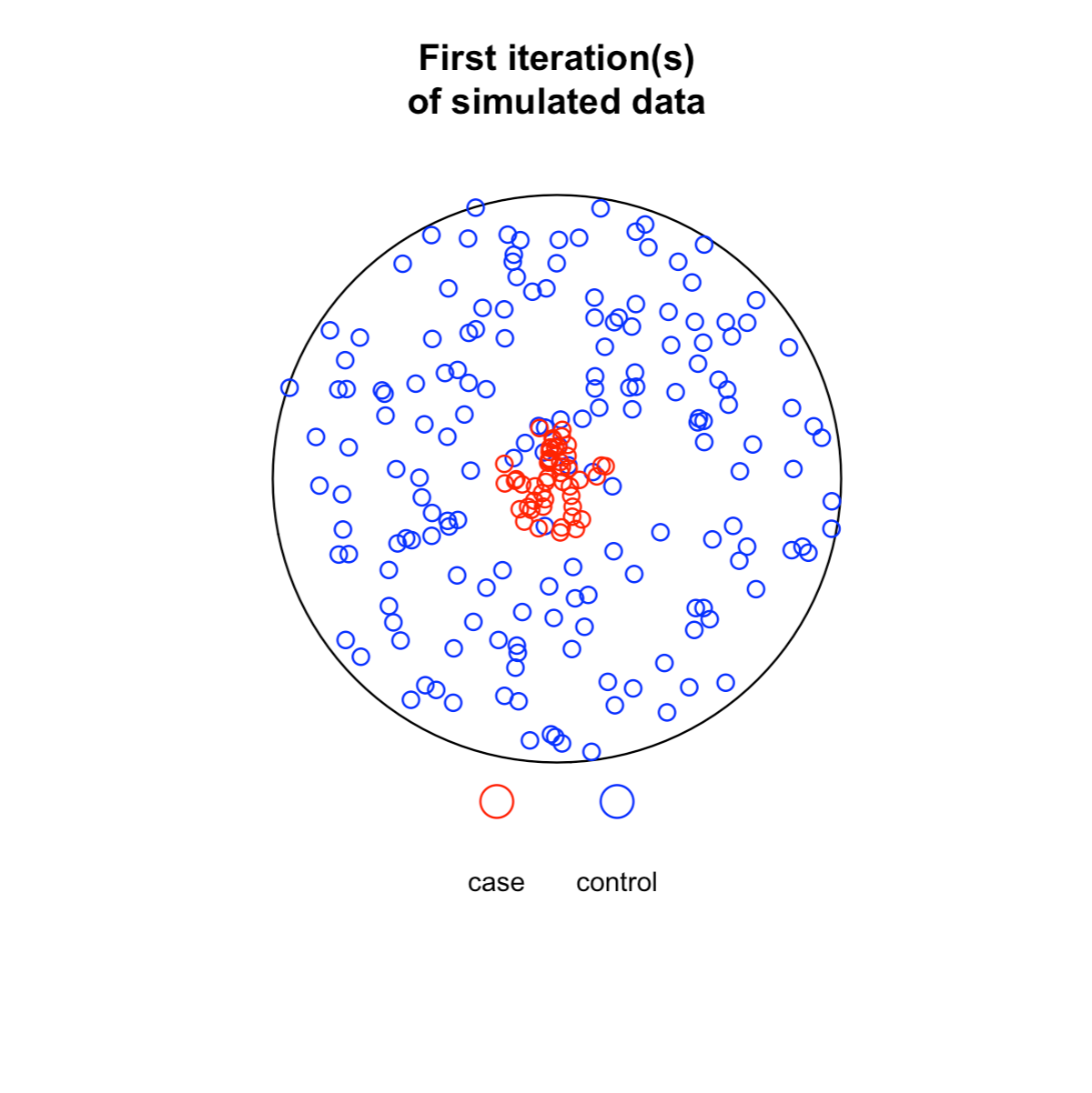
# Circular window with radius 0.5
# Uniform case sampling within a disc of radius of 0.1 at the center of the window
# Complete Spatial Randomness control sampling
# 20% prevalence (n = 300 total locations)
# Statistical power to detect both case and control relative clustering
# 100 simulations (more recommended for power calculation)
unit.circle <- spatstat.geom::disc(radius = 0.5, centre = c(0.5,0.5))
foo <- spatial_power(win = unit.circle,
sim_total = 100,
x_case = 0.5,
y_case = 0.5,
samp_case = "uniform",
samp_control = "CSR",
r_case = 0.1,
n_case = 50,
n_control = 250)
# ----------------------- #
# Outputs from iterations #
# ----------------------- #
# Mean and standard deviation of simulated sample sizes and bandwidth
mean(foo$n_con); stats::sd(foo$n_con) # controls
mean(foo$n_cas); stats::sd(foo$n_cas) # cases
mean(foo$bandw); stats::sd(foo$bandw) # bandwidth of case density (if fixed, same for control density)
# Global Test Statistics
## Global maximum relative risk: Null hypothesis is mu = 1
stats::t.test(x = foo$s_obs, mu = 0, alternative = "two.sided")
## Integral of log relative risk: Null hypothesis is mu = 0
stats::t.test(x = foo$t_obs, mu = 1, alternative = "two.sided")
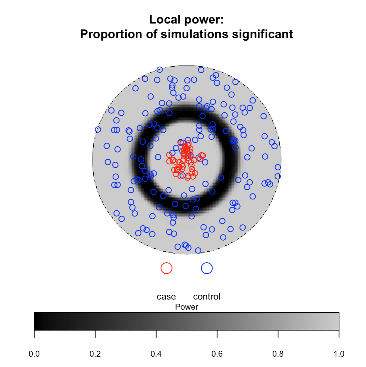
# ----------------- #
# Run spatial_plots #
# ----------------- #
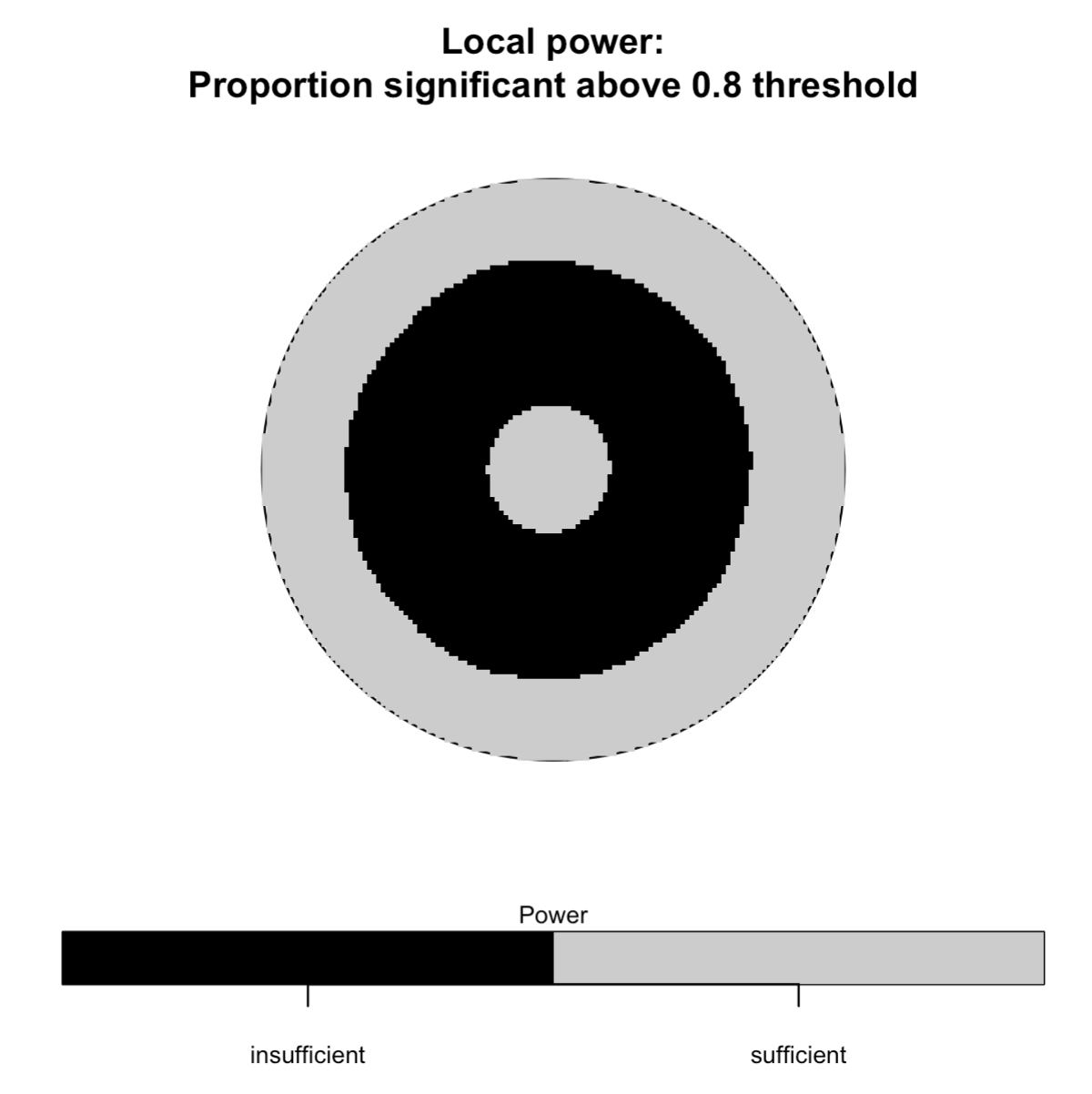
# Statistical power for case-only clustering (one-tailed test)
spatial_plots(foo)
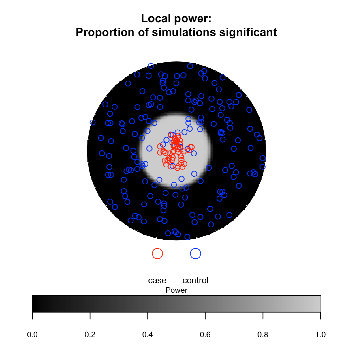
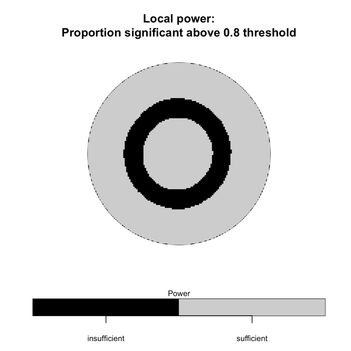
# Statistical power for case clustering and control
clustering (two-tailed test)
## Only showing second and third plot
spatial_plots(foo, cascon = TRUE)
# --------------------------- #
# Multiple Testing Correction #
# --------------------------- #
# Same parameters as above
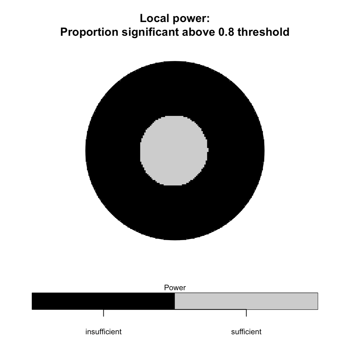
# Apply a conservative Bonferroni correction
set.seed(1234) # reset RNG
# Run spatial_power()
foo <- spatial_power(win = unit.circle,
sim_total = 100,
x_case = 0.5,
y_case = 0.5,
samp_case = "uniform",
samp_control = "CSR",
r_case = 0.1,
n_case = 50,
n_control = 250,
alpha = 0.05,
p_correct = "FDR")
median(foo$alpha) # critical p-value of 3e-6
# Run spatial_plots() for case-only clustering
## Only showing third plot
spatial_plots(foo, cascon = TRUE)