
![]()
![]()
To cite stagedtrees in publications use:
Carli F, Leonelli M, Riccomagno E, Varando G (2022). “The R Package stagedtrees for Structural Learning of Stratified Staged Trees.” Journal of Statistical Software, 102(6), 1-30. doi: 10.18637/jss.v102.i06 (URL: https://doi.org/10.18637/jss.v102.i06).
@Article{,
    title = {The {R} Package {stagedtrees} for Structural Learning of Stratified Staged Trees},
    author = {Federico Carli and Manuele Leonelli and Eva Riccomagno and Gherardo Varando},
    journal = {Journal of Statistical Software},
    year = {2022},
    volume = {102},
    number = {6},
    pages = {1--30},
    doi = {10.18637/jss.v102.i06},
}stagedtrees is a package that implements staged event trees, a probability model for categorical random variables.
#stable version from CRAN
install.packages("stagedtrees")

#development version from github
# install.packages("devtools")
devtools::install_github("gherardovarando/stagedtrees")With the stagedtrees package it is possible to fit (stratified) staged event trees to data, use them to compute probabilities, make predictions, visualize and compare different models.
A staged event tree object (sevt class) can be initialized as the full (saturated) or as the fully independent model with, respectively, the functions indep and full. It is possible to build a staged event tree from data stored in a data.frame or a table object.
# Load the PhDArticles data
data("Titanic")

# define order of variables
order <- c("Sex", "Age",  "Class", "Survived")

# Independence model
mod_indep <- indep(Titanic, order)
mod_indep
#> Staged event tree (fitted)
#> Sex[2] -> Age[2] -> Class[4] -> Survived[2]
#> 'log Lik.' -5773.349 (df=7)

# Full (saturated) model
mod_full <- full(Titanic, order)
mod_full
#> Staged event tree (fitted)
#> Sex[2] -> Age[2] -> Class[4] -> Survived[2]
#> 'log Lik.' -5151.517 (df=30)By default staged trees object are defined assuming structural zeros in the contingency tables. This is implemented by joining all unobserved situations in particular stages (named by default "UNOBSERVED") which are, by default, ignored by other methods and functions (see the ignore argument in ?stages_bhc or ?plot.sevt).
## there are no observations for Sex=Male (Female), Age = Child, Class = Crew
get_stage(mod_full, c("Male", "Child", "Crew"))
#> [1] "UNOBSERVED"

## and obviously
prob(mod_full, c(Age = "CHild", CLass = "Crew"))
#> [1] 0It is possible to initialize a staged tree without structural zeros by setting the argument join_unobserved=FALSE. In that case, it can be useful to set lambda > 0 to avoid problems with probabilities on unobserved situations.
stagedtrees implements methods to perform automatic model selection. All methods can be initialized from an arbitrary staged event tree object.
This methods perform optimization for a given score using different heuristics.
stages_hc(object, score, max_iter, scope, ignore, trace)mod1 <- stages_hc(mod_indep)
mod1
#> Staged event tree (fitted)
#> Sex[2] -> Age[2] -> Class[4] -> Survived[2]
#> 'log Lik.' -5161.242 (df=18)stages_bhc(object, score, max_iter, scope, ignore, trace)mod2 <- stages_bhc(mod_full)
mod2
#> Staged event tree (fitted)
#> Sex[2] -> Age[2] -> Class[4] -> Survived[2]
#> 'log Lik.' -5157.759 (df=19)stages_fbhc(object, score, max_iter, scope, ignore, trace)mod3 <- stages_fbhc(mod_full, score = function(x) -BIC(x))
mod3
#> Staged event tree (fitted)
#> Sex[2] -> Age[2] -> Class[4] -> Survived[2]
#> 'log Lik.' -5164.708 (df=18)stages_bj(object, distance, thr, scope, ignore, trace)mod4 <- stages_bj(mod_full)
mod4
#> Staged event tree (fitted)
#> Sex[2] -> Age[2] -> Class[4] -> Survived[2]
#> 'log Lik.' -5170.769 (df=21)stages_hclust(object, distance, k, method, ignore, limit, scope)mod5 <- stages_hclust(mod_full,
k = 2,
distance = "totvar",
method = "mcquitty")
mod5
#> Staged event tree (fitted)
#> Sex[2] -> Age[2] -> Class[4] -> Survived[2]
#> 'log Lik.' -5241.629 (df=12)stages_kmeans(object, k, algorithm, ignore, limit, scope, nstart)mod6 <- stages_kmeans(mod_full,
k = 2,
algorithm = "Hartigan-Wong")
mod6
#> Staged event tree (fitted)
#> Sex[2] -> Age[2] -> Class[4] -> Survived[2]
#> 'log Lik.' -5241.629 (df=12)|> (or %>%)The new native pipe operator |> (or the one from the magrittr package) can be used to combine various model selection algorithms.
model <- Titanic |> full(lambda = 1) |> stages_hclust() |> stages_hc()

## extract a sub_tree and join two stages
small_model <- model |> subtree(path = c("Crew"))  |>
join_stages("Survived", "3", "7")Obtain marginal (or conditionals) probabilities with the prob function.
# estimated probability of c(Sex = "Male", Class = "1st")
# using different models
prob(mod_indep, c(Sex = "Male", Class = "1st"))
#> [1] 0.1161289
prob(mod3, c(Sex = "Male", Class = "1st"))
#> [1] 0.08110992
Or for a data.frame of observations:
obs <- expand.grid(mod_full$tree[c(1,3)])
p <- prob(mod2, obs)
cbind(obs, P = p)
#>      Sex Class          P
#> 1   Male   1st 0.08110992
#> 2 Female   1st 0.06655023
#> 3   Male   2nd 0.08273137
#> 4 Female   2nd 0.04675523
#> 5   Male   3rd 0.23097925
#> 6 Female   3rd 0.08978404
#> 7   Male  Crew 0.39164016
#> 8 Female  Crew 0.01044980
Conditional probabilities can be obtained via the conditional_on argument.
A staged event tree object can be used to make predictions with the predict method. The class variable can be specified, otherwise the first variable (root) in the tree will be used.
## check accuracy over the Titanic data
titanic_df <- as.data.frame(Titanic)
predicted <- predict(mod3, class = "Survived", newdata = titanic_df)
table(predicted, titanic_df$Survived)
#>
#> predicted No Yes
#>       No   7   7
#>       Yes  7   7
Conditional probabilities (or log-) can be obtained setting prob = TRUE:
## obtain estimated conditional probabilities in mod3
predict(mod3, newdata = titanic_df[1:3,], prob = TRUE)
#>       Male   Female
#> 1 0.587156 0.412844
#> 2 0.587156 0.412844
#> 3 0.587156 0.412844sample_from(mod4, 5)
#> Sex Age Class Survived
#> 1 Male Adult 2nd No
#> 2 Female Adult 3rd No
#> 3 Female Adult 2nd No
#> 4 Male Adult 2nd No
#> 5 Male Adult Crew No# stages
stages(mod1, "Age")
#> [1] "3" "1"
# summary
summary(mod1)
#> Call:
#> stages_hc(mod_indep)
#> lambda: 0
#> Stages:
#> Variable: Sex
#> stage npaths sample.size Male Female
#> 1 0 2201 0.7864607 0.2135393
#> ------------
#> Variable: Age
#> stage npaths sample.size Child Adult
#> 3 1 1731 0.03697285 0.9630272
#> 1 1 470 0.09574468 0.9042553
#> ------------
#> Variable: Class
#> stage npaths sample.size 1st 2nd 3rd Crew
#> 1 2 109 0.05504587 0.2201835 0.7247706 0.00000000
#> 3 1 1667 0.10497900 0.1007798 0.2771446 0.51709658
#> 4 1 425 0.33882353 0.2188235 0.3882353 0.05411765
#> ------------
#> Variable: Survived
#> stage npaths sample.size No Yes
#> 4 5 174 0.02298851 0.9770115
#> 1 2 910 0.77472527 0.2252747
#> UNOBSERVED 2 0 NA NA
#> 6 3 371 0.60377358 0.3962264
#> 7 2 630 0.85873016 0.1412698
#> 5 2 116 0.13793103 0.8620690
#> ------------
# confidence intervals
confint(mod1, parm = "Age")
#> 2.5 % 97.5 %
#> Age=Child|3 0.02808370 0.0458620
#> Age=Adult|3 0.95413800 0.9719163
#> Age=Child|1 0.06914343 0.1223459
#> Age=Adult|1 0.87765407 0.9308566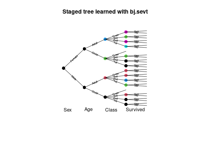
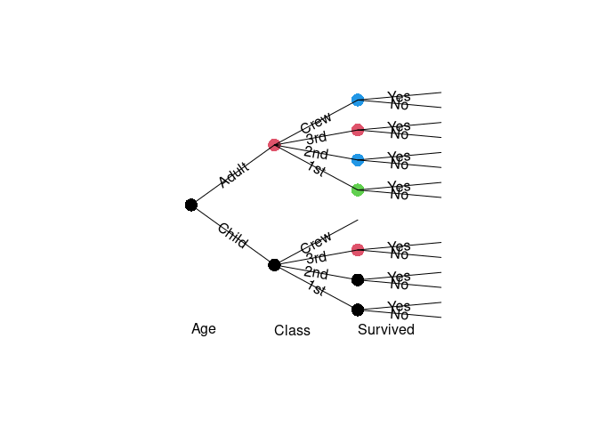
By default stages associated with the unobserved situations are not plotted, if the model has been created with join_unobserved = TRUE. But we can plot also the unobserved stages in a specific color.
plot(stndnaming(mod5, uniq = TRUE),
     main = "Staged tree learned with stages_hclust
     (unobserved in grey)",
     ignore = FALSE, ## do not ignore stages
     col = function(stages) ifelse(stages=="UNOBSERVED", "grey", stages),
     cex_label_edges = 0.6, cex_nodes = 1.5)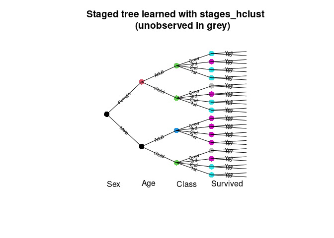
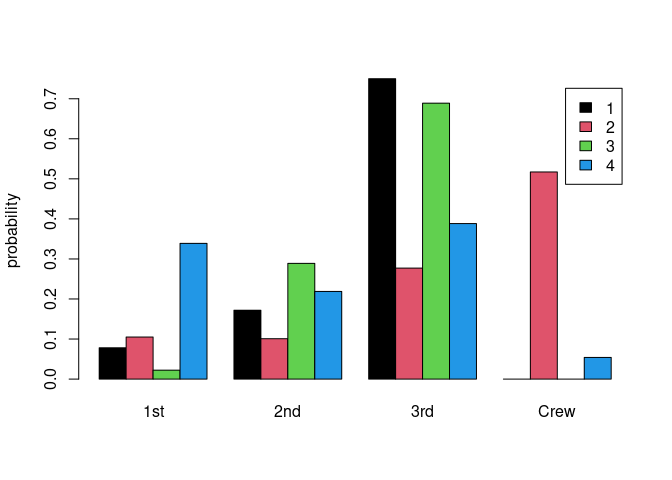
The method barplot.sevt creates a bar plot for the conditional probabilities of a variable.
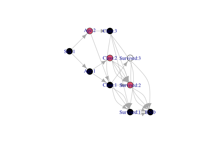
Plotting CEG requires the igraph package.
From a staged evnt tree a subtree can be extracted, the resulting model is ar staged event tree in the remaining variables.
compare_stages(mod1, mod4)
#> [1] FALSE

compare_stages(mod1, mod4, method = "hamming", plot = TRUE,
             cex_label_nodes = 0, cex_label_edges = 0)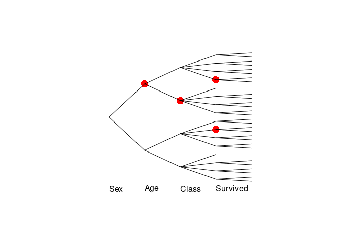
#> [1] FALSE

hamming_stages(mod1, mod4)
#> [1] 4

difftree <- compare_stages(mod1, mod4, method = "stages", plot = FALSE,
             return_tree = TRUE)

difftree$Married
#> NULLBIC(mod_indep, mod_full, mod1, mod2, mod3, mod4, mod5)
#> df BIC
#> mod_indep 7 11600.57
#> mod_full 30 10533.93
#> mod1 18 10461.02
#> mod2 19 10461.76
#> mod3 18 10467.96
#> mod4 21 10503.17
#> mod5 12 10575.62mod1a <- join_stages(mod1, "Class", "3", "4")
lr_test(mod1a, mod1)
#> Likelihood-ratio test
#>
#> Sex[2] -> Age[2] -> Class[4] -> Survived[2]
#> Model 1: mod1a
#> Model 2: mod1
#> #Df LogLik Df Chisq Pr(>Chisq)
#> 1 15 -5359.6
#> 2 18 -5161.2 3 396.65 < 2.2e-16 ***
#> ---
#> Signif. codes: 0 '***' 0.001 '**' 0.01 '*' 0.05 '.' 0.1 ' ' 1