
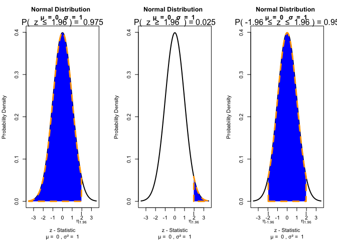
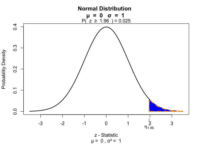
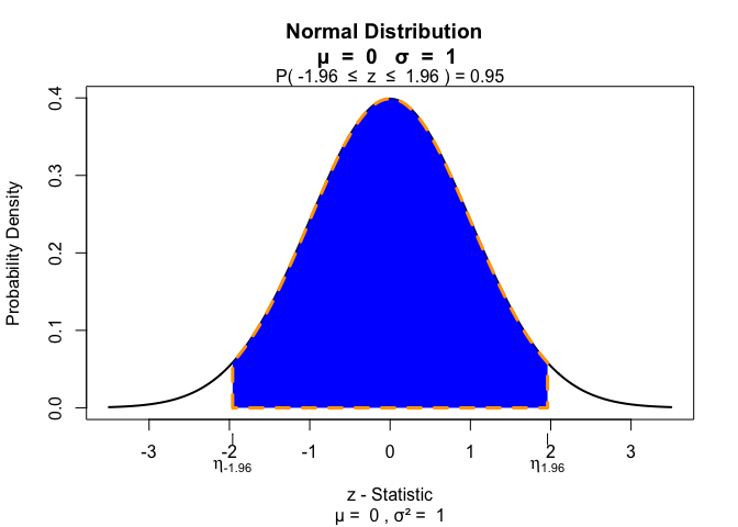
The goal of visualize is to graph the pdf or pmf and highlight what area or probability is present in user defined locations. Visualize is able to provide lower tail, bounded, upper tail, and two tail calculations. Supports strict and equal to inequalities. Also provided on the graph is the mean and variance of the distribution.
You can install the released version of visualize from CRAN with:
And the development version from GitHub with:
To use visualize, load the package with:
Then, construct a graph by following the visualize.dist() pattern. For example, the normal distribution can be shown with:
The parameters of the distribution can also be modified. Take for example the Binomial distribution.
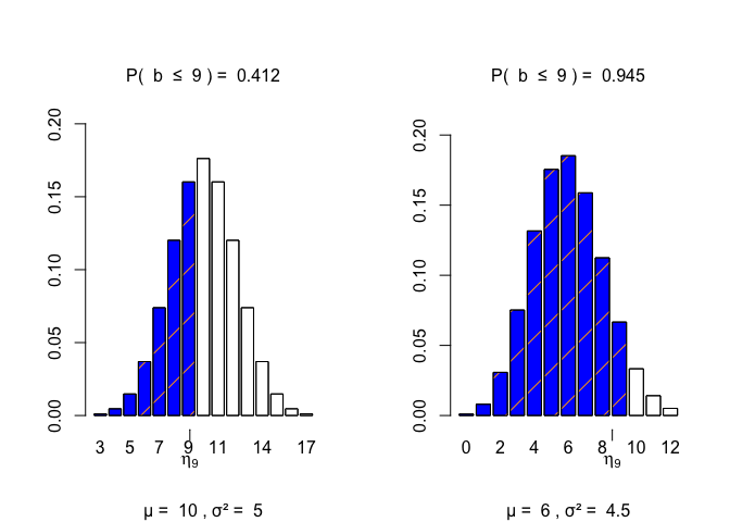
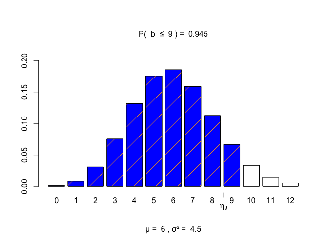
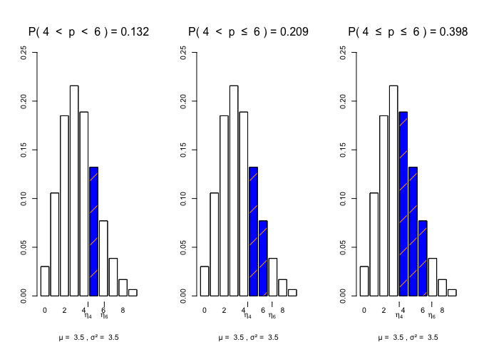
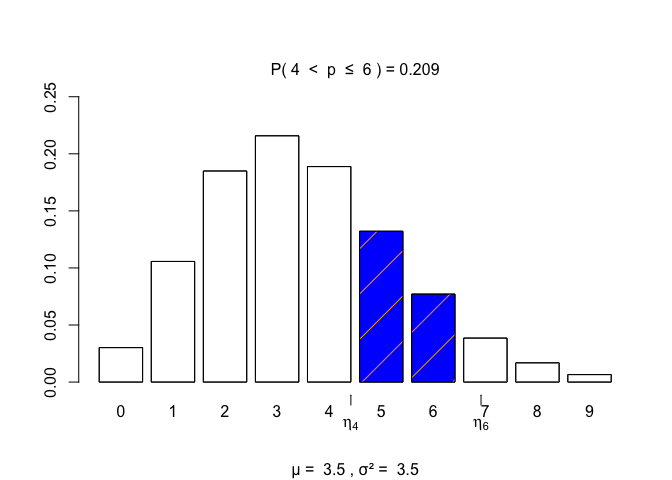
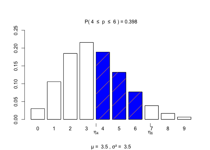
Discrete distributions can also handle a level of strict (<, >) or equal to (<=, >=) inequality.
James Joseph Balamuta
visualize packageTo ensure future development of the package, please cite visualize package if used during an analysis or simulation study. Citation information for the package may be acquired by using in R:
MIT License