
“Waywiser” is an old-timey name for a surveyor’s wheel, a device that makes measuring long distances easier than with measurement tools like a ruler or yardstick. The waywiser R package makes measuring model performance on spatial data easier, extending the yardstick R package to incorporate measures of spatial autocorrelation provided by spdep.
You can install waywiser from CRAN via:
install.packages("waywiser")You can install the development version of waywiser from GitHub with:
# install.packages("devtools")
devtools::install_github("mikemahoney218/waywiser")Let’s walk through how we can use waywiser to find local indicators of spatial autocorrelation for a very simple model. First things first, let’s load a few libraries:
# waywiser itself, of course:
library(waywiser)
# For the %>% pipe and mutate:
library(dplyr)
We’ll be working with the guerry data from the sfdep
package, fitting a linear model to associate crimes against persons with
literacy. Let’s load the data now:
data(guerry, package = "sfdep")We’ll fit a simple linear model relating crimes against persons with
literacy, and then generate predictions from that model. We can use
ww_local_moran_i() to calculate the local spatial
autocorrelation of our residuals at each data point:
guerry %>%
  mutate(pred = predict(lm(crime_pers ~ literacy, .))) %>%
  ww_local_moran_i(crime_pers, pred)
#> # A tibble: 85 × 4
#>    .metric       .estimator .estimate                                   geometry
#>    <chr>         <chr>          <dbl>                             <MULTIPOLYGON>
#>  1 local_moran_i standard      0.530  (((381847 1762775, 381116 1763059, 379972…
#>  2 local_moran_i standard      0.858  (((381847 1762775, 381116 1763059, 379972…
#>  3 local_moran_i standard      0.759  (((381847 1762775, 381116 1763059, 379972…
#>  4 local_moran_i standard      0.732  (((381847 1762775, 381116 1763059, 379972…
#>  5 local_moran_i standard      0.207  (((381847 1762775, 381116 1763059, 379972…
#>  6 local_moran_i standard      0.860  (((381847 1762775, 381116 1763059, 379972…
#>  7 local_moran_i standard      0.692  (((381847 1762775, 381116 1763059, 379972…
#>  8 local_moran_i standard      1.69   (((381847 1762775, 381116 1763059, 379972…
#>  9 local_moran_i standard     -0.0109 (((381847 1762775, 381116 1763059, 379972…
#> 10 local_moran_i standard      0.710  (((381847 1762775, 381116 1763059, 379972…
#> # … with 75 more rows
If you’re familiar with spdep, you can probably guess that waywiser
is doing something under the hood here to calculate which of
our observations are neighbors, and how to create spatial weights from
those neighborhoods. And that guess would be right – waywiser is making
use of two functions, ww_build_neighbors() and
ww_build_weights(), in order to automatically calculate
spatial weights for calculating metrics:
ww_build_neighbors(guerry)
#> Neighbour list object:
#> Number of regions: 85
#> Number of nonzero links: 420
#> Percentage nonzero weights: 5.813149
#> Average number of links: 4.941176

ww_build_weights(guerry)
#> Characteristics of weights list object:
#> Neighbour list object:
#> Number of regions: 85
#> Number of nonzero links: 420
#> Percentage nonzero weights: 5.813149
#> Average number of links: 4.941176
#>
#> Weights style: W
#> Weights constants summary:
#>    n   nn S0      S1       S2
#> W 85 7225 85 37.2761 347.6683
These functions aren’t always the best way to calculate spatial weights for your data, however. As a result, waywiser also lets you specify your own weights directly:
weights <- guerry %>%
  sf::st_geometry() %>%
  sf::st_centroid() %>%
  spdep::dnearneigh(0, 97000) %>%
  spdep::nb2listw()

weights
#> Characteristics of weights list object:
#> Neighbour list object:
#> Number of regions: 85
#> Number of nonzero links: 314
#> Percentage nonzero weights: 4.346021
#> Average number of links: 3.694118
#>
#> Weights style: W
#> Weights constants summary:
#>    n   nn S0       S1       S2
#> W 85 7225 85 51.86738 348.7071

guerry %>%
  mutate(pred = predict(lm(crime_pers ~ literacy, .))) %>%
  ww_local_moran_i(crime_pers, pred, weights)
#> # A tibble: 85 × 4
#>    .metric       .estimator .estimate                                   geometry
#>    <chr>         <chr>          <dbl>                             <MULTIPOLYGON>
#>  1 local_moran_i standard    0.530    (((381847 1762775, 381116 1763059, 379972…
#>  2 local_moran_i standard    0.794    (((381847 1762775, 381116 1763059, 379972…
#>  3 local_moran_i standard    0.646    (((381847 1762775, 381116 1763059, 379972…
#>  4 local_moran_i standard    0.687    (((381847 1762775, 381116 1763059, 379972…
#>  5 local_moran_i standard    0.207    (((381847 1762775, 381116 1763059, 379972…
#>  6 local_moran_i standard    1.49     (((381847 1762775, 381116 1763059, 379972…
#>  7 local_moran_i standard    0.692    (((381847 1762775, 381116 1763059, 379972…
#>  8 local_moran_i standard    1.69     (((381847 1762775, 381116 1763059, 379972…
#>  9 local_moran_i standard   -0.000610 (((381847 1762775, 381116 1763059, 379972…
#> 10 local_moran_i standard    0.859    (((381847 1762775, 381116 1763059, 379972…
#> # … with 75 more rows
Or as a function, which lets you use custom weights with other
tidymodels functions like fit_resamples():
weights_function <- function(data) {
  data %>%
    sf::st_geometry() %>%
    sf::st_centroid() %>%
    spdep::dnearneigh(0, 97000) %>%
    spdep::nb2listw()
}

guerry %>%
  mutate(pred = predict(lm(crime_pers ~ literacy, .))) %>%
  ww_local_moran_i(crime_pers, pred, weights_function)
#> # A tibble: 85 × 4
#>    .metric       .estimator .estimate                                   geometry
#>    <chr>         <chr>          <dbl>                             <MULTIPOLYGON>
#>  1 local_moran_i standard    0.530    (((381847 1762775, 381116 1763059, 379972…
#>  2 local_moran_i standard    0.794    (((381847 1762775, 381116 1763059, 379972…
#>  3 local_moran_i standard    0.646    (((381847 1762775, 381116 1763059, 379972…
#>  4 local_moran_i standard    0.687    (((381847 1762775, 381116 1763059, 379972…
#>  5 local_moran_i standard    0.207    (((381847 1762775, 381116 1763059, 379972…
#>  6 local_moran_i standard    1.49     (((381847 1762775, 381116 1763059, 379972…
#>  7 local_moran_i standard    0.692    (((381847 1762775, 381116 1763059, 379972…
#>  8 local_moran_i standard    1.69     (((381847 1762775, 381116 1763059, 379972…
#>  9 local_moran_i standard   -0.000610 (((381847 1762775, 381116 1763059, 379972…
#> 10 local_moran_i standard    0.859    (((381847 1762775, 381116 1763059, 379972…
#> # … with 75 more rows
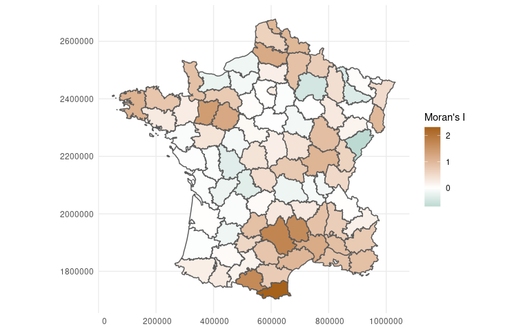
Providing custom weights also lets us use
ww_local_moran_i_vec to add a column to our original data
frame with our statistic, which makes plotting using our original
geometries easier:
library(ggplot2)

weights <- ww_build_weights(guerry)

guerry %>%
  mutate(pred = predict(lm(crime_pers ~ literacy, .)),
         .estimate = ww_local_moran_i_vec(crime_pers, pred, weights)) %>%
  sf::st_as_sf() %>%
  ggplot(aes(fill = .estimate)) +
  geom_sf() +
  scale_fill_gradient2(
    "Moran's I",
    low = "#018571",
    mid = "white",
    high = "#A6611A"
  )
This makes it easy to see what areas are poorly represented by our model, which might lead us to identify ways to improve our model or help us identify caveats and limitations of the models we’re working with.
This project is released with a Contributor Code of Conduct. By contributing to this project, you agree to abide by its terms.
If you think you have encountered a bug, please submit an issue.
Please include a reprex (a minimal, reproducible example) to clearly communicate about your code.